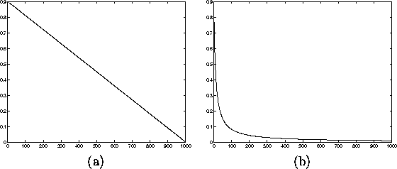
Learning rate is a decreasing function of time. Two forms that are
commonly used are a linear function of time and a function that is
inversely proportional to the time t. These are illustrated in the
Figure 2.7. Linear alpha function (a) decreases to zero
linearly during the learning from its initial value whereas the
inverse alpha function (b) decreases rapidly from the initial value
Both the functions in the Figure have the initial value of 0.9. The
initial values for ![]() must be determined. Usually, when using a
rapidly decreasing inverse alpha function, the initial values can be
larger than in the linear case. The learning is usually performed in
two phases. On the first round relatively large initial alpha values
are used (
must be determined. Usually, when using a
rapidly decreasing inverse alpha function, the initial values can be
larger than in the linear case. The learning is usually performed in
two phases. On the first round relatively large initial alpha values
are used ( ![]() ) whereas small initial alpha
values (
) whereas small initial alpha
values ( ![]() ) are used during the other round.
This corresponds to first tuning the SOM approximately to the same
space than the inputs and then fine-tuning the map. There are several
rules-of-thumb for picking suitable values. These have been found
through experiments and can be found in the monograph by Kohonen
[20].
) are used during the other round.
This corresponds to first tuning the SOM approximately to the same
space than the inputs and then fine-tuning the map. There are several
rules-of-thumb for picking suitable values. These have been found
through experiments and can be found in the monograph by Kohonen
[20].

Figure 2.7: Learning rates as functions of time
Alpha values are defined to be
![]()
for the linear case and
![]()
for the inverse function. C can be, for example C = rlen / 100. rlen is the running length of the training, or number of samples fed to the network. These are the values used in the programming package SOM_PAK [21].
By choosing a suitable initial learning rate and a suitable form for the learning rate function, we can considerably affect the result.