Nonlinear factor analysis and nonlinear state-space models can be seen as special cases of Bayesian networks where the linearity assumption is relaxed. Aside from these two, there are lots of possibilities to build the model structure that defines the dependencies between the parameters and the data. To be able to manage the variety, a modular software package using C++/Python called the Bayes Blocks (Valpola et al., 2003a) has been created. It is introduced in Publication I and in an earlier conference paper by Valpola et al. (2001).
The design principles for Bayes Blocks have been the following. Firstly, we use standardised building blocks that can be connected rather freely and can be learned with local learning rules, i.e. each block only needs to communicate with its neighbours. Secondly, the system should work with very large scale models. Computational complexity is linear with respect to the number of data samples and connections in the model.
The building blocks include Gaussian variables, summation,
multiplication, and nonlinearity. The framework does not make much difference in
parameters
 and latent variables
 , the former are
represented with scalars and the latter as vectors. Variational
Bayesian learning provides a cost function which can be used for
updating the variables as well as optimising the model structure. The
derivation of the cost function, as well as learning and inference
rules, is automatic which means that the user only needs to define the
connections between the blocks.
, the former are
represented with scalars and the latter as vectors. Variational
Bayesian learning provides a cost function which can be used for
updating the variables as well as optimising the model structure. The
derivation of the cost function, as well as learning and inference
rules, is automatic which means that the user only needs to define the
connections between the blocks.
The Gaussian node is a variable node and the basic element in building
hierarchical models. Figure 4.4 (leftmost subfigure)
shows the schematic diagram of the Gaussian node. Its output is the
value of a Gaussian random variable  , which is conditioned by the
inputs
, which is conditioned by the
inputs  and
and  . Denote generally by
 the
probability density function of a Gaussian random variable
the
probability density function of a Gaussian random variable  having
the mean
having
the mean  and variance
 . Then the conditional
probability function of the variable is
. Then the conditional
probability function of the variable is
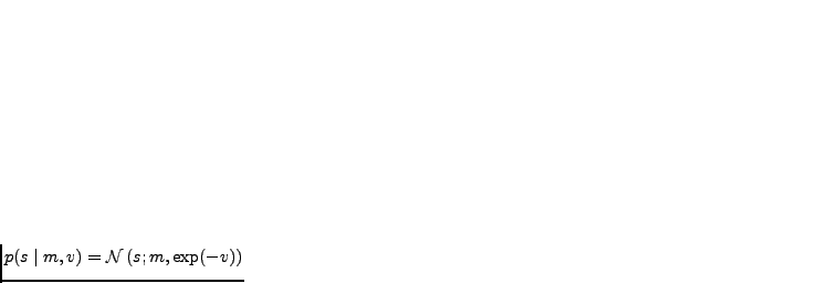 . As a generative model, the Gaussian node takes
its mean input and adds to it Gaussian noise (or innovation) with
variance
. As a generative model, the Gaussian node takes
its mean input and adds to it Gaussian noise (or innovation) with
variance  .
.
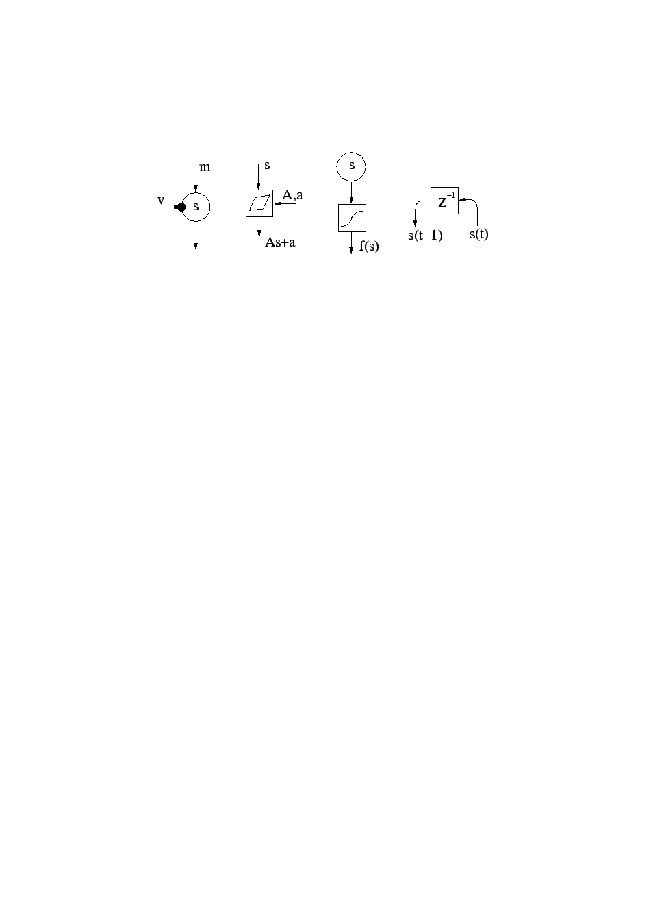 |
The addition and multiplication nodes are used for summing and multiplying variables. These standard mathematical operations are typically used to construct linear mappings between the variables. A nonlinear computation node can be used for constructing nonlinear mappings between the variable nodes. The delay operation can be used to model dynamics. Harva et al. (2005) implements several new blocks including mixture-of-Gaussians and rectified Gaussians. Harva and Kabán (2005) use the rectified Gaussian node to create a factor model with non-negativity constraints and Nolan et al. (2006) applies Bayes Blocks in an astronomical problem.
Nodes propagate certain expectations about their state to their
neighbours in the network. For variable nodes in a network, update
rules for the posterior approximation  that minimise the cost
function
that minimise the cost
function
 given that of all the other variables stays
constant, have been derived. The updates are very simple since the
posterior approximation is of a very simple form: It is a Gaussian
with a diagonal covariance matrix.
given that of all the other variables stays
constant, have been derived. The updates are very simple since the
posterior approximation is of a very simple form: It is a Gaussian
with a diagonal covariance matrix.
Winn and Bishop (2005) introduce an algorithm called variational message passing with close similarities with Bayes Blocks. It does not allow for nonlinearities or variance modelling (see the following section), but on the other hand, it handles discrete variables more freely. It also allows for a posterior approximation factorised such that disjoint groups of variables are independent, but dependencies within the group are modelled. Variational message passing updates the posterior approximation of one factor at a time using VB learning. Note that the best properties of Bayes Blocks and variational message passing could be combined.
Similar models can be studied also with rather different posterior approximations. Spiegelhalter et al. (1995) introduce the BUGS software package that uses Gibbs sampling (see Section 2.5.4) for Bayesian inference. The package supports mixture models, nonlinearities, and non-stationary variance. A thorough experimental comparison to Bayes Blocks would be very valuable.
 . Third subfigure: A nonlinearity
 is applied immediately after a Gaussian variable. The
rightmost subfigure: Delay operator delays a time-dependent signal
by one time unit.
is applied immediately after a Gaussian variable. The
rightmost subfigure: Delay operator delays a time-dependent signal
by one time unit.