In many models, variances are assumed to have constant values although this assumption is often unrealistic in practice. Joint modelling of means and variances is difficult in many learning approaches, because it can give rise to infinite probability densities. In Bayesian methods where sampling is employed, the difficulties with infinite probability densities are avoided, but these methods are not efficient enough for very large models. The Bayes Blocks allow to build hierarchical or dynamical models for the variance.
The Bayes Blocks framework was used by Valpola et al. (2004) to jointly model both variances and means in biomedical MEG data. The same approach can be used to translate any model for a mean to a model for a variance, so a large number of models in the literature could be explored as models for variance as well.
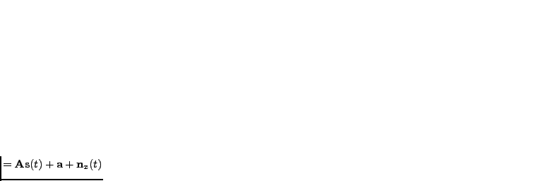
The left subfigure of Figure 4.5 shows how linear
state-space model (see Section 3.1.6) is built using Bayes
Blocks. It can be extended
into a model for both means and variances as depicted
graphically in the right subfigure of Figure 4.5. The variance sources
 characterise the innovation process of
 , in
effect telling how much the signal differs from the predicted one but
not in which direction it is changing. Both regular sources
and variance sources
are modelled dynamically by using
one-step recursive prediction model for them. The model
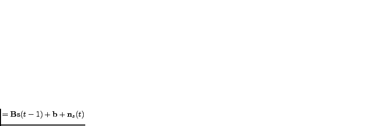
equations are:
, in
effect telling how much the signal differs from the predicted one but
not in which direction it is changing. Both regular sources
and variance sources
are modelled dynamically by using
one-step recursive prediction model for them. The model
equations are:
 |
 |
(4.14) |
 |
 |
(4.15) |
 |
![$\displaystyle = \mathcal{N}\left(n_{si}(t);0,\exp\left[-u_i(t)\right]\right)$](img264.png) |
(4.16) |
 |
 |
(4.17) |
 , the
, the  th component of the noise
vector
th component of the noise
vector
 , is determined by the variance source
  .
.
![\includegraphics[width=0.2\textwidth]{kalman}](img269.png)
![\includegraphics[width=0.45\textwidth]{vardyn}](img270.png)
|