Computational Performance

In the first set of experiments we compared the computational performance of different algorithms on PCA with missing values. The root mean square (rms) error is measured on the training data, $\operatorname{E}_O=\sqrt{\frac{1}{\vert O\vert}\sum_{(i,j) \in O} e_{ij}^2}$. All experiments were run on a dual cpu AMD Opteron SE 2220 using Matlab.

First, we tested the imputation algorithm. The first iteration where the missing values are replaced with zeros, was completed in 17 minutes and led to $E_O=0.8527$. This iteration was still tolerably fast because the complete data matrix was sparse. After that, it takes about 30 hours per iteration. After three iterations, $E_O$ was still 0.8513.

Using the EM algorithm by [11], the E-step (updating $\mathbf{S}$) takes 7 hours and the M-step (updating $\mathbf{A}$) takes 18 hours. (There is some room for optimization since we used a straightforward Matlab implementation.) Each iteration gives a much larger improvement compared to the imputation algorithm, but starting from a random initialization, EM could not reach a good solution in reasonable time.

We also tested the subspace learning algorithm described in Section 3 with and without the proposed speed-up. Each run of the algorithm with different values of the speed-up parameter $\alpha$ was initialized in the same starting point (generated randomly from a normal distribution). The learning rate $\gamma$ was adapted such that if an update decreased the cost function, $\gamma$ was multiplied by 1.1. 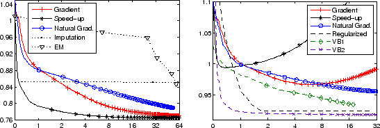Each time an update would increase the cost, the update was canceled and $\gamma$ was divided by 2. Figure 1 (left) shows the learning curves for basic gradient descent, natural gradient descent, and the proposed speed-up with the best found parameter value $\alpha=0.625$. The proposed speed-up gave about a tenfold speed-up compared to the gradient descent algorithm even if each iteration took longer. Natural gradient was slower than the basic gradient. Table 1 gives a summary of the computational complexities.

Figure 1: Left: Learning curves for unregularized PCA (Section 3) applied to the Netflix data: Root mean-square error on the training data $E_O$ is plotted against computation time in hours. Right: The root mean square error on the validation data $E_V$ from the Netflix problem during runs of several algorithms: basic PCA (Section 3), regularized PCA (Section 4) and VB (Section 4). VB1 has some parameters fixed (see [12]) while VB2 updates all the parameters. The time scales are linear below 1 and logarithmic above 1.

Table 1: Summary of the computational performance of different methods on the Netflix problem. Computational complexities (per iteration) assume naïve computation of products and inverses of matrices and ignores the computation of SVD in the imputation algorithm. While the proposed speed-up makes each iteration slower than the basic gradient update, the time to reach the error level 0.85 is greatly diminished.

Method	Complexity	Seconds/Iter	Hours to $E_O=0.85$
Gradient	$O(Nc+nc)$	58	1.9
Speed-up	$O(Nc+nc)$	110	0.22
Natural Grad.	$O(Nc+nc^2)$	75	3.5
Imputation	$O(nd^2)$	110000	$\gg 64$
EM	$O(Nc^2+nc^3)$	45000	58