Regularization

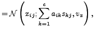
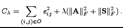
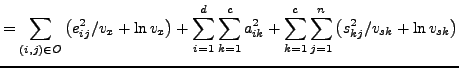
A popular way to regularize ill-posed problems is penalizing the use of large parameter values by adding a proper penalty term into the cost function; see for example [3]. In our case, one can modify the cost function in Eq. (2) as follows:

$$C_{\lambda} = \sum_{(i,j) \in O} e_{ij}^2 + \lambda ( \lVert\mathbf{A}\rVert _F^2 + \lVert\mathbf{S}\rVert _F^2 ) \, .$$ (17)

This has the effect that the parameters that do not have significant evidence will decay towards zero.

A more general penalization would use different regularization parameters $\lambda$ for different parts of $\mathbf{A}$ and $\mathbf{S}$. For example, one can use a $\lambda_{k}$ parameter of its own for each of the column vectors $\mathbf{a}_k$ of $\mathbf{A}$ and the row vectors $\mathbf{s}_k$ of $\mathbf{S}$. Note that since the columns of $\mathbf{A}$ can be scaled arbitrarily by rescaling the rows of $\mathbf{S}$ accordingly, one can fix the regularization term for $\mathbf{a}_k$, for instance, to unity.

An equivalent optimization problem can be obtained using a probabilistic formulation with (independent) Gaussian priors and a Gaussian noise model:

$$p(x_{ij} \mid \mathbf{A},\mathbf{S}) = \mathcal{N}\left(x_{ij};\sum_{k=1}^c a_{ik}s_{kj},v_x\right),$$ (18)

$$p(a_{ik}) = \mathcal{N}\left(a_{ik};0,1\right), \quad p(s_{kj}) = \mathcal{N}\left(s_{kj};0,v_{sk}\right) \, ,$$ (19)

where $\mathcal{N}\left(x;m,v\right)$ denotes the random variable $x$ having a Gaussian distribution with the mean $m$ and variance $v$. The regularization parameter $\lambda_{k}$ = $v_{sk}/v_x$ is the ratio of the prior variances $v_{sk}$ and $v_x$. Then, the cost function (ignoring constants) is minus logarithm of the posterior for $\mathbf{A}$ and $\mathbf{S}$:

$$C_ = \sum_{(i,j) \in O} \left( e_{ij}^2/v_x + \ln v_x \right) + \s... ...a_{ik}^2 + \sum_{k=1}^c\sum_{j=1}^n \left(s_{kj}^2/v_{sk} + \ln v_{sk} \right)$$ (20)

An attractive property of the Bayesian formulation is that it provides a natural way to choose the regularization constants. This can be done using the evidence framework (see, e.g., [3]) or simply by minimizing $C_$BR by setting $v_x$, $v_{sk}$ to the means of $e_{ij}^2$ and $s_{kj}^2$ respectively. We will use the latter approach and refer to it as regularized PCA.

Note that in case of joint optimization of $C_$BR w.r.t. $a_{ik}$, $s_{kj}$, $v_{sk}$, and $v_x$, the cost function (20) has a trivial minimum with $s_{kj}=0$, $v_{sk}\rightarrow 0$. We try to avoid this minimum by using an orthogonalized solution provided by unregularized PCA from the learning rules (14) and (15) for initialization. Note also that setting $v_{sk}$ to small values for some components $k$ is equivalent to removal of irrelevant components from the model. This allows for automatic determination of the proper dimensionality $c$ instead of discrete model comparison (see, e.g., [13]). This justifies using separate $v_{sk}$ in the model in (19).