Problem setting

The working hypothesis to be tested was that the NDFA algorithm should be able to find a representation for the observations which facilitates the prediction of the observations, i.e., a representation where modelling the dynamics of the underlying data generating process is easier than directly for the original observations.

  

Figure 3: Time evolution of the state resulting from the Lorenz system with $\sigma = 3$, $\rho = 26.5$ and $\beta = 1$.

Data was generated by first defining the underlying dynamic process and then mapping some of the states of the process onto observations by one of the random MLP networks which were used in [4].

The underlying dynamic process was constructed by combining three independent dynamic processes. One of the processes was harmonic oscillator with angular velocity 1/3. The harmonic oscillator has a two-dimensional state representation and linear dynamics. Notice, however, that if the harmonic oscillator is modelled with linear dynamics, the gain has to be exactly one. Otherwise the oscillations will either decay or grow exponentially for gains less than or greater than one, respectively. A robust model for a harmonic oscillator with a constant amplitude therefore needs to be nonlinear.

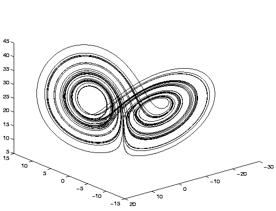
The two other processes were chosen to be Lorenz processes [5]. The Lorenz system has a three-dimensional state space whose dynamics is governed by the following set of differential equation:

$$\frac{dz_1}{dt} \sigma(z_2 - z_1)$$ = (16)

$$\frac{dz_2}{dt} \rho z_1 - z_2 - z_1 z_3$$ = (17)

$$\frac{dz_3}{dt} z_1 z_2 - \beta z_3$$ = (18)

The parameter vectors $[\sigma \ \ \rho \ \ \beta]$ for the processes were chosen to be $[3 \ \ 26.5 \ \ 1]$ and $[4 \ \ 30 \ \ 1]$. The time evolution of the state for the first Lorenz process is shown in figure 3.

The ability to find the underlying factors which have generated the observations was already demonstrated in [4]. To make the problem more difficult, one dimension of each of the three elementary processes was hidden. As the original process has a total of eight states, five states are left from which the data was generated nonlinearly. In [4], some of the experiments used a random MLP network with inverse hyperbolic sine activation functions to generate ten-dimensional observations from five inputs. The same MLP network was used here. Like in [4], the data set consisted of 1000 observation.

  

Figure 4: Each plot shows a time series. The eight plots on the top show the eight states on which the dynamics of the underlying process is defined. The process is composed of two Lorenz processes, each of which has three states, and a harmonic oscillator which has two states. Five projections from the eight states are used for generating the observations. These are shown in the middle. The ten plots on the bottom of the figure are the noisy observations which are obtained by instantaneous nonlinear mapping from the five projections.

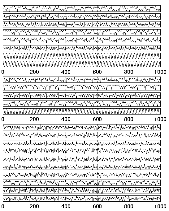
Figure 4 shows the eight states of the underlying dynamical system, the five projections made from them and the noisy observations obtained from the projections by the random MLP network. The standard deviation of the observation noise was 0.1 while the standard deviation of the signal was normalised to unity.