 |
A convenient by-product of using a factorial approximation of the posterior density in ensemble learning is that unused parts of the model are effectively pruned away. The reason for this is that the learning process aims at fitting the approximation to the true posterior. It is usually the case that the model has some indeterminacies, which basically means that several different values for the variables in the model yield exactly the same probability for the observations. It is then impossible to determine the variables based on observations.
For ensemble learning this can be a benefit because it allows a choice of parameter values which make the factorial assumption of the posterior density more valid. In other words, extra degrees of freedom in the model can be used for improving the approximation of the posterior density.
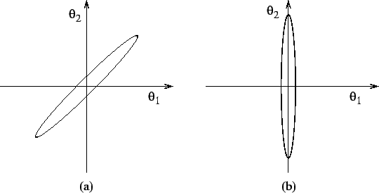
If the model has more parameters or factors than are required, some of them are not well determined which will be reflected in having equal posterior and prior distributions. In a general case where the variables have posterior correlations, there are some directions in the variable space which are well determined and others which are not. Figure 8a gives an example of such a situation. The difference of the two parameters is well determined while the value of their sum is uncertain.
 |
If indeterminacies have produced degrees of freedom which allow rotation of the parameter space, then ensemble learning will try to make the variables posteriorly independent as shown in figure 8b. This means that the variables tend to be either well determined or not determined at all. Equation (21) which is the Kullback-Leibler information between the prior and approximated posterior density of a variable can be used for assessing whether the variable is actually used by the model. If the posterior is close to the prior, the variable is not well determined. From the coding point of view, equation (21) can also be interpreted as the number of bits used by the model to represent that variable. If very few bits are used to represent a variable, it is not needed by the model and can be pruned away without affecting the model.