The preliminary winning strengths ![]() were defined by
equation 3.7
were defined by
equation 3.7

We shall rewrite this
where ![]() and
and ![]() . This equation has to be solved numerically, since
. This equation has to be solved numerically, since
![]() appear in both sides of the equation, and it is impossible to
find the solution in a closed form. The computation only needs to be
done for the neurons in the set of winners, and therefore n equals
the number of winners.
appear in both sides of the equation, and it is impossible to
find the solution in a closed form. The computation only needs to be
done for the neurons in the set of winners, and therefore n equals
the number of winners.
Newton's method is often a good choice when one has to numerically
solve equations. If we denote ![]() , then solving equation 4.1 is
equivalent to finding the root of
, then solving equation 4.1 is
equivalent to finding the root of ![]() . Finding the root using
Newton's method requires the computation of the inverse of the Jacobian
matrix of
. Finding the root using
Newton's method requires the computation of the inverse of the Jacobian
matrix of ![]() , however. It is a n by n matrix, because
both vectors
, however. It is a n by n matrix, because
both vectors ![]() and
and ![]() have n elements. In some
cases it is possible to find an efficient way to compute the inverse
of the Jacobian. This is possible, if the Jacobian is for example close
to diagonal matrix. In our case the Jacobian is not at all close to
diagonal matrix, and it does not seem to have any other properties
which would allow us to compute the inverse efficiently.
have n elements. In some
cases it is possible to find an efficient way to compute the inverse
of the Jacobian. This is possible, if the Jacobian is for example close
to diagonal matrix. In our case the Jacobian is not at all close to
diagonal matrix, and it does not seem to have any other properties
which would allow us to compute the inverse efficiently.
We are going to solve the equation 4.1 by using another
popular method: fixed point iteration. If we have an equation
of the form x = f(x) we can try to find the solution simply by
iterating x(t+1) = f(x(t)). This is the standard fixed point
iteration. Suppose ![]() is a solution satisfying
is a solution satisfying ![]() .
The iteration converges to
.
The iteration converges to ![]() only if
only if ![]() . Notice that
if the derivative f' is negative, the value x(t) oscillates around
the solution
. Notice that
if the derivative f' is negative, the value x(t) oscillates around
the solution ![]() , and if the derivative is positive, the value
x(t) changes monotonically. The closer the derivative is to zero
the faster is the convergence.
, and if the derivative is positive, the value
x(t) changes monotonically. The closer the derivative is to zero
the faster is the convergence.
It is also possible to speed up the convergence by modifying the
iteration. Aitken extrapolation formula [Atkinson, 1989, page 86,]
makes the assumption that the values x(t) form a geometric series if
we use the standard fixed point iteration. This assumption is usually
valid at least when x(t) are close to the solution ![]() and the
derivative f'(x(t)) is approximately constant. We shall start from
x(t) and compute the values x(t+1) and x(t+2) by using the
standard fixed point iteration. Then we shall assume that x(t),
x(t+1) and x(t+2) are consecutive values in a geometric series
which converges to
and the
derivative f'(x(t)) is approximately constant. We shall start from
x(t) and compute the values x(t+1) and x(t+2) by using the
standard fixed point iteration. Then we shall assume that x(t),
x(t+1) and x(t+2) are consecutive values in a geometric series
which converges to ![]() , and solve an estimate
, and solve an estimate ![]() . We can
then assign
. We can
then assign ![]() and iterate the process.
and iterate the process.
If we know that f'(x) < 0 for all x, it is also possible to derive
an alternative modification which can speed up the convergence. Let
us write ![]() , and consider
the iteration process
, and consider
the iteration process ![]() . For a proper
choice of
. For a proper
choice of ![]() the derivative
the derivative ![]() , and the convergence
is at least quadratic. Even if
, and the convergence
is at least quadratic. Even if ![]() , by choosing
, by choosing
![]() sufficiently small the iteration can be made to converge
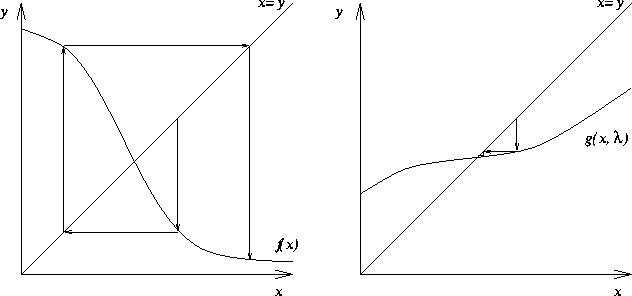
(see figure 4.1). We shall find a way to adapt the
sufficiently small the iteration can be made to converge
(see figure 4.1). We shall find a way to adapt the
![]() so that the derivative of
so that the derivative of ![]() with respect to
x will become as close to zero as possible.
with respect to
x will become as close to zero as possible.
If ![]() is too large, the derivative is less than zero and x(t)
oscillates. This will manifest itself as an alternating sign of the
differences of consecutive values of x(t). If
is too large, the derivative is less than zero and x(t)
oscillates. This will manifest itself as an alternating sign of the
differences of consecutive values of x(t). If ![]() is too
small, the derivative is greater than zero and x(t) changes
monotonically. This too can be detected from the sign of the
differences, which stays unchanged. We can now formulate a rule for
adapting the
is too
small, the derivative is greater than zero and x(t) changes
monotonically. This too can be detected from the sign of the
differences, which stays unchanged. We can now formulate a rule for
adapting the ![]() during iteration. After each iteration of
x(t) we shall calculate the sign of x(t)-x(t-1). If it has
changed after last iteration, we shall decrease
during iteration. After each iteration of
x(t) we shall calculate the sign of x(t)-x(t-1). If it has
changed after last iteration, we shall decrease ![]() , otherwise
we shall increase it. The use of
, otherwise
we shall increase it. The use of ![]() speeds up convergence and
allows convergence even if
speeds up convergence and
allows convergence even if ![]() .
.
In our case the equation 4.1 is a system of equations.
We can still use the Aitken extrapolation formula or the adaptation
rule for ![]() proposed above, but this time we have to apply the
modifications to each of the functions
proposed above, but this time we have to apply the
modifications to each of the functions ![]() separately. Both of the
modified methods and the standard fixed point iteration were tested in
simulations. The iterated function was like that in
equation 4.1. There were ten neurons, and the values
separately. Both of the
modified methods and the standard fixed point iteration were tested in
simulations. The iterated function was like that in
equation 4.1. There were ten neurons, and the values
![]() were sampled from an even distribution between -4 and 0.
The closer the values were to zero the better the convergence was.
The distribution used in this test can be thought of as a sort of
worst case, because normally the values are not this small.
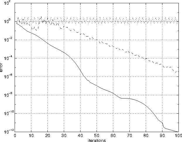
Figure 4.2 shows a typical test run. The standard
method did not converge at all. The iteration using Aitken
extrapolation formula usually converged, but much more slowly than the
proposed method, which converged in all tests. The good performance
of the proposed method is probably due to the fact that all partial
derivatives
were sampled from an even distribution between -4 and 0.
The closer the values were to zero the better the convergence was.
The distribution used in this test can be thought of as a sort of
worst case, because normally the values are not this small.
Figure 4.2 shows a typical test run. The standard
method did not converge at all. The iteration using Aitken
extrapolation formula usually converged, but much more slowly than the
proposed method, which converged in all tests. The good performance
of the proposed method is probably due to the fact that all partial
derivatives ![]() since
since ![]() . Therefore the value of each of the variables
. Therefore the value of each of the variables ![]() typically
oscillate in the standard fixed point iteration, and the use of
adaptive
typically
oscillate in the standard fixed point iteration, and the use of
adaptive ![]() can efficiently dampen the oscillation.
can efficiently dampen the oscillation.

Figure 4.1:
In the left, fixed point iteration does not converge to the
solution ![]() , because
, because ![]() . The derivative is
negative, and therefore the derivative of a new function
. The derivative is
negative, and therefore the derivative of a new function ![]() can be made zero by a
proper choose of
can be made zero by a
proper choose of ![]() . In the right,
. In the right, ![]() ,
and
,
and ![]() .
.

Figure 4.2:
The proposed modified fixed point iteration method using adaptive
![]() (solid line) has been compared with the standard method
(dotted line) and Aitken extrapolation formula (dashed line). The
proposed method has converged much more rapidly than the iteration
using Aitken extrapolation formula, while the standard method has
not converged at all.
(solid line) has been compared with the standard method
(dotted line) and Aitken extrapolation formula (dashed line). The
proposed method has converged much more rapidly than the iteration
using Aitken extrapolation formula, while the standard method has
not converged at all.