Definition of the Model

  

Figure 3: The mapping from sources to observations is modelled by the familiar MLP network. The sources are on the top layer and observations in the bottom layer. The middle layer consists of hidden neurons each of which computes a nonlinear function of the inputs

The schematic structure of the mapping is shown in Fig. 3. The nonlinearity of each hidden neuron is the hyperbolic tangent, which is the same as the usual logistic sigmoid except for a scaling. The equation defining the mapping is

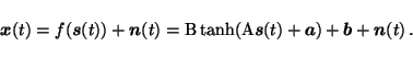$$\vec{x}(t) = f(\vec{s}(t)) + \vec{n}(t) = \mathrm{B} \tanh( \mathrm{A} \vec{s}(t) + \vec{a}) + \vec{b} + \vec{n}(t) \, .$$ (3)

The matrices A and B are the weights of first and second layer and $\vec{a}$ and $\vec{b}$ are the corresponding biases.

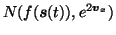
The noise is assumed to be independent and Gaussian and therefore the probability distribution of x(t) is

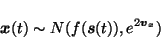$$\vec{x}(t) \sim N(f(\vec{s}(t)), e^{2\vec{v}_x})$$ (4)

Each component of the vector $\vec{v}_x$ gives the log-std of the corresponding component of $\vec{x}(t)$.

The sources are assumed to have zero mean Gaussian distributions and again the variances are parametrised by log-std $\vec{v}_s$.

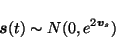$$\vec{s}(t) \sim N(0, e^{2\vec{v}_s})$$ (5)

Since the variance of the sources can vary, variance of the weights A on the first layer can be fixed to a constant, which we choose to be one, without loosing any generality from the model. This is not case for the second layer weights. Due to the nonlinearity, the variances of the outputs of the hidden neurons are bounded from above and therefore the variance of the second layer weights cannot be fixed. In order to enable the network to shut off extra hidden neurons, the weights leaving one hidden neuron share the same variance parameter.

$$\mathrm{B} \sim N(0, e^{2\vec{v}_B})$$ (6)

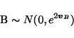
The elements of the matrix B are assumed to have a zero mean Gaussian distribution with individual variances for each column and thus the dimension of the vector $\vec{v}_B$ is the number of hidden neurons. Both biases $\vec{a}$ and $\vec{b}$ have Gaussian distributions parametrised by mean and log-std.

The distributions are summarised in (7)-(12).

   

$$\vec{x}(t) \sim N(f(\vec{s}(t)), e^{2\vec{v}_x})$$ (7)

$$\vec{s}(t) \sim N(0, e^{2\vec{v}_s})$$ (8)

$$\sim$$ A N(0, 1) (9)

$$\sim N(0, e^{2\vec{v}_B})$$ B (10)

$$\vec{a} \sim$$ N(m_a, e^2v_a) (11)

$$\vec{b} \sim$$ N(m_b, e^2v_b) (12)

The distributions of each set of log-std parameters are modelled by Gaussian distributions whose parameters are usually called hyperparameters.

 

$$\vec{v}_x \sim$$ N(m_vx, e^2v_vx) (13)

$$\vec{v}_s \sim$$ N(m_vs, e^2v_vs) (14)

$$\vec{v}_B \sim$$ N(m_vB, e^2v_vB) (15)

The prior distributions of m_a, v_a, m_b, v_b and the six hyperparameters $m_{v_s}, \ldots, v_{v_B}$ are assumed to be Gaussian with zero mean and standard deviation 100, i.e., the priors are assumed to be very flat.