Model structure

According to the general FA model the data has been generated by factors s through mapping f:

 

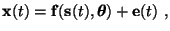$$\mathbf{x}(t) = \mathbf{f}(\mathbf{s}(t), \boldsymbol{\theta}) + \mathbf{e}(t) \ ,$$ (3)

where x is a data vector, s is a factor vector, $\boldsymbol{\theta}$ is a parameter vector and e is a noise vector. The factors and the noise are assumed to be independent and Gaussian:

$$\sim N(0,\sigma_{l}^{2})$$ s_l(t) (4)

$$\sim N(0,\xi_{k}^{2})$$ e_k(t)

The linear mapping f used in FA is

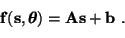$$\mathbf{f}(\mathbf{s}, \boldsymbol{\theta}) = \mathbf{A}\mathbf{s} + \mathbf{b}\ .$$ (5)

The model is similar to principal component analysis except that FA includes the noise term and the factors have a Gaussian distribution. In NFA, the function f is allowed to be nonlinear. We use the method proposed in [6], where the MLP network

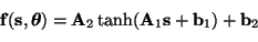$$\mathbf{f}(\mathbf{s}, \boldsymbol{\theta}) = \mathbf{A}_{2} \tanh(\mathbf{A}_{1}\mathbf{s}+\mathbf{b}_{1})+\mathbf{b}_{2}$$ (6)

is used to model the nonlinearity. The parameter vector  $\boldsymbol{\theta}$ contains both A and b.

In NFA the data is modelled by a high dimensional manifold created by function  f from a prior Gaussian distribution. It can be compared to the self-organising map (SOM) [5], but the number of parameters scale more like in FA. The SOM scales exponentially as function of the dimensionality of the underlying data manifold. A small number of parameters keeps the modelled manifold smooth. We find the parameter vector  $\boldsymbol{\theta}$ using ensemble learning.