 |
For the fine tuning of the HMMs several methods have been suggested based on heuristics resembling the LVQ2 [Bahl et al., 1988,Mizuta and Nakajima, 1990,Juang and Katagiri, 1992,Galindo, 1995]. The idea is first to train the HMMs normally and then improve their performance by some additional corrective iterations (last phase in Figure 3). The formulation of the training method is here more difficult than in the initialization phase where the labels of the training samples are predetermined. The segmentation of the training samples that determines to which state each data vector belongs, which is the basis of the LVQ training, is assumed to vary while the models gradually improve. The correct state segmentation of the data depends on the HMMs and vice versa. Thus the tuning of the model and the segmentation of the data must be developed together so that the tuning and the segmentation operations take turns and the process advances iteratively.
 |
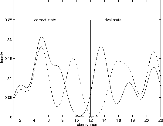
Since the segmentation of the data is not predefined but improves gradually while the training proceeds, it is difficult to determine the optimal size for the stochastic learning steps. There are two conflicting aims, to weight more the gradient directions given by the later better segmentations, but still to force the process to converge at a reasonable speed. The learning from recognition errors by corrective tuning relates the models rather closely to the training data so that for finite data the long-run behavior of the learning process might not give the desired result. The solution tested in Publication 2 was to use an exponential decay for the learning rate and to check the change of the error rate on a separate data set after each epoch through the training set. Using then all the test runs for all the available speakers the suitable average amount of epochs was determined to be the limit after which no average improvement was detected. The corrective tuning method based on the LVQ2 learning law (9) is described in Publication 2. Figure 8 illustrates a simple example of the tuning process.
Contrary to most of the other corrective training methods, the LVQ2 based method used here does not relate the individual parameter adjustments to the exact extent of the difference of the resulting probabilities of the rival HMM state sequences. These whole word path probability differences follow from the straight derivation of the loss function, e.g. see [Rainton and Sagayama, 1992]. Anyhow, here only the given learning rate and the local differences of the likelihood values provided by the rival mixtures determine the extent of the parameter adjustments. This is to avoid the risk of improper step sizes, which might follow from the occurrence of both severe and slight errors in the same word. Another difference is that the method applies the LVQ2-type learning law [Kohonen, 1990b] only to the detected actual misrecognition cases. Thus no tuning occurs, if the decoded phonemes match to the correct phoneme segmentation obtained by constraining the Viterbi search to the known correct transcription from the word list. This restriction is to avoid the risk of forcing some parameters out of the useful range by too frequent penalizations.
In Publications 1 and 2 brief experimental results are given on applying the corrective tuning for CDHMMs and SCHMMs after the normal maximum likelihood training by Baum-Welch or Viterbi training. In Publications 4 and 6 more thorough experiments are presented for MDHMMs by trying different input features and speech data. The conclusions are that, on the average, the recognition results have improved significantly by the corrective tuning. However, the new segmental LVQ3 method (see the next section) can give the same improvement faster and more conveniently by using only one training algorithm.