Selective accuracy.

High accuracy for the density modeling for MDHMMs is required only for the most likely states for good discrimination between the closest candidates. For the other states a quick approximation providing only the correct order of magnitude suffices.

For the mixture Gaussian probability estimates it is characteristic that each Gaussian provides a good accuracy only for samples near the centroid and that the total density estimate is strongly dominated by the few Gaussians close to the sample. To get more Gaussians to the areas where many input vectors fall, it is important that the point density of the Gaussian units reflect as well as possible the density of the input space. This ensures then the maximal resource utilization where it is most beneficial. The more units there are in the important areas the more robust and accurate PDF approximation can be expected. If there were only one unit, the small random effects due to its distance from the observation and its state-dependent weight may influence excessively to the accuracy of the PDF estimate. The exact form of the kernel functions will have less significance, as well, when the amount of participating kernels increases. This can be of importance for strongly non-Gaussian densities.

  

Figure 5: The average distances (here called quantization errors) of the five best matching units in the Gaussian codebook of the correct phoneme. The correct phoneme means the phoneme for which the feature vector is segmented at the end of the HMM training. The labels of the curves indicate the training methods that have been used. The initialization options K-means and SOM are indicated by 'km' and 'som', respectively. The segmental training options are correspondingly abbreviated as 'skm' and 'ssom'. The 'ssom_apx' means that the approximative topological K-best search (see Section 3.2.5) is used in the testing. To see the development of the relative differences of the compared training methods the average quantization error d of each of the top 5 units is plotted using the relative difference of errors to the default method (d - d₀)/d₀ , here d₀ is from 'som+ssom'. The purpose of this figure is to show that adapting the neighborhoods will bring more units near the input vectors, in average.

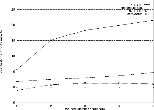
Compared to the codebooks trained without neighborhoods, e.g. trained by K-means, the accuracy obtained by the best-matching Gaussian can be worse, but the next (K-1) best matches will be better. Figure 5 shows the relative difference of the distances of the nearest Gaussians for differently trained density codebooks. From all the curves having the SOM initialization, the later segmental K-means training will provide the BMU most accurately.

For following sections there are a couple of further notes from Figure 5. If the segmental LVQ3 training (Section 3.3.4) is applied after the SOM initialization the corresponding curve almost equals the 'som+skm' curve. This is not surprising, because both training methods rely on the smoothing obtained only by the initialization and because the discriminative adaptations are not expected to affect the average distances. For Section 3.2.5 it is noteworthy that the quality of the approximative search on the SOM codebook is rather close to the original, and decreases slowly when going further from the best match. This indicates that the PDF approximation will not dramatically mess the total values of the output densities for the expected closest states.