Figure 2.1: Black box
Artificial neural networks are adaptive models that can learn from the data and generalize things learned. They extract the essential characteristics from the numerical data as opposed to memorizing all of it. This offers a convenient way to reduce the amount of data as well as to form a implicit model without having to form a traditional, physical model of the underlying phenomenon. In contrast to traditional models, which are theory-rich and data-poor, the neural networks are data-rich and theory-poor in a way that a little or no a priori knowledge of the problem is present [8]. Neural networks can be used for building mappings from inputs to ouputs of these kind of black boxes. The behavior of a black box system is not usually known. This is illustrated in Figure 2.1. These kind of systems occur often in practice.
Neural networks are models as such. These models can be used to characterize the general case of the phenomenon at hand giving us the ideas how the phenomenon behaves in practice.
Artificial neural networks or shortly neural networks have been quite promising in offering solutions to problems, where traditional models have failed or are very complicated to build. Due to the non-linear nature of the neural networks, they are able to express much more complex phenomena than some linear modeling techniques.
Kohonen divides artificial neural networks into three categories [20]:
In signal transfer networks, the input signal is transformed into an output signal. The signal traverses the network and undergoes a signal transformation of some kind. The network has usually a set of pre-defined basis functions, which are parametrized. The learning in these networks corresponds to changing parameters of these basis functions. Some examples are the multi-layer perceptron (MLP) networks that are taught with error back propagation algorithm (BP) and radial basis function (RBF) networks. More about these network models can be found in textbooks, for example in [3], [12].
In state transition networks the dynamic behavior of the network is essential. Given an input, the network converges to a stable state, which, hopefully, is a solution to a problem presented to it. Examples are Hopfield networks and Boltzmann machines. See [12] for reference.
In competitive learning networks, or self-organizing networks, all the neurons of the network receive the same input. The cells have lateral competition and the one with most activity ``wins''. Learning is based on the concept of winner neurons. A representative example of a network based on competitive learning is the Self-Organizing Map. The monograph by Kohonen [20] is the most complete book about this particular network model.
Learning in artificial neural networks is done in terms of adaptation of the network parameters. Network parameters are changed according to pre-defined equations called the learning rules. The learning rules may be derived from pre-defined error measures or may be inspired by biological systems. An example of an error measure in a network based on supervised learning could be the squared error between the output of the model and the desired output. This requires knowledge of the desired value for a given input. Learning rules are written so that the iterative learning process minimizes the error measure. Minimization might be performed by gradient descent optimization methods, for instance. In the course of learning, the residual between the model output and the desired output decreases and the model learns the relation between the input and the output.
The training must be stopped at the right time. If training continues for too long, it results in overlearning. Overlearning means that the neural network extracts too much information from the individual cases forgetting the relevant information of the general case.

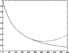
Figure 2.2: The model residual versus time for the training and the
testing set
In the Figure 2.2 we can see two different curves. The difference between the network output and desired output, or the model residual is plotted as a function of training time. We can see that the model residual decreases for the training set marked with a solid line but starts to increase for the testing set marked with the dashed line. When the network starts to learn the characteristics on individual samples rather than the characteristics of the general phenomenon, the model residual for the testing set starts to increase. The model is departing from the general structure of the problem to learning about the individual cases instead.
Usually, the neural network performance is tested with a testing set which is not part of the training set. The testing set can be seen as the representative cases of the general phenomenon. If the network performs well on the testing set, it can be expected to perform well on the general case, as well.
Cross-validation methods can also be used to avoid overlearning. In cross-validation, we switch the places of the training set and the testing set and compare the performance of the resulting networks.
It is essential to understand the characteristics of a particular neural network model before using it. In this way, one can avoid many pitfalls of neural networks.
In the next section, the attention is on a particular neural network model called the Self-Organizing Map.