Finding the underlying process

The NDFA algorithm was used for learning a dynamic model of the observations. Several different random initialisations of the MLP networks and structures of the model were tested. For the first 500 iterations, the concatenated vector ${\mathbf{y}}(t) = [{\mathbf{x}}(t-2)^T \ \ldots \ {\mathbf{x}}(t+2)^T]^T$ was used instead of x(t) as the observation vectors. After that, y(t) was replaced by x(t) and the observation MLP was reduced accordingly. The cost function was found to be minimised by a model where there were ten factors and both the observation MLP network and the factor dynamics MLP network had one hidden layer of 30 neurons.

  

Figure 5: The ten plots on the top show the factors s(t) after 7500 iterations and the ten plots on the bottom show the factors after 600,000 iterations. The first 1000 values have been estimated based on the observations and the following 1000 values have been predicted using s(t) = g(s(t-1)), i.e., without the innovation process.

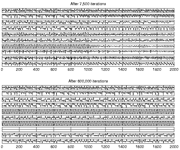
After 7500 iterations the model had learned a dynamic process which was able to represent the observations. The standard deviation of the observations was estimated to be 0.106 on the average which is in reasonably good agreement with the actual value of 0.1. In order to test the quality of the dynamic model learned by the algorithm, 1000 new values were predicted for the factors using the estimated mapping g. The factors are shown in the upper part of figure 5.

The experiments with NLFA reported in [4] indicated that 7500 iterations were sufficient for learning the factors and the observation mapping. It turned out that more iterations are needed to fully learn the underlying dynamical process. Most of the learning was finished after 100,000 iterations, but some progress was observed even after 600,000 iterations. The simulation was not continued beyond that, however. In any case, the experiment confirms that ensemble learning is robust against overlearning, i.e., there is no need to control the complexity of the resulting mappings by early stopping of learning. The lower part of figure 5 shows the factors in the end of learning.

Visual inspection of the plots in figure 5 confirms that the NDFA algorithm has been able to capture the characteristics of the dynamics of the data-generating process. It also shows that only nine out of ten factors are actually used in the end. However, it is difficult to compare the estimated dynamics with the original by looking only at the predicted factors s(t). This is because the model learned by the NDFA uses a state representation which differs from the original.

  

Figure 6: The original eight-dimensional state of the underlying process used for generating the observations is reconstructed from the predicted factors s(t) shown in figure 5. After 7500 iterations the model can follow the dynamics for a while and after 600,000 iterations the essential characteristics of the dynamics are captured with high fidelity as can be seen by comparing the original latent variables ( $1 \leq t \leq 1000$) to the following 1000 predicted states.

Two processes can be considered equivalent if their state representations differ only by an invertible nonlinear transformation. As the original underlying states of the process are known, it is possible to examine the dynamics in the original state space. An MLP network was used for finding the mapping from the learned ten-dimensional factors to the original eight-dimensional states. The mapping was then used for visualising the dynamics in the original state space.

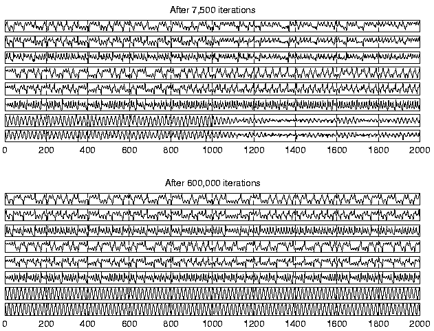
Figure 6 shows the reconstruction of the original states made from the predicted states s(t). First of all, it is evident that the factors contain all the required information about the state of the underlying process because the reconstructions are quite good for $1 \leq t \leq 1000$ even after 7500 iterations. Initially the dynamics is not modelled accurately enough to simulate the long term behaviour of the process, but in the end, the dynamics of all three underlying subprocesses are captured.