Multi-layer perceptron networks

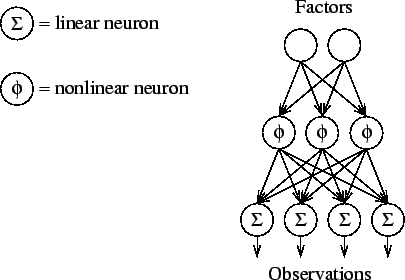
The nonlinear model is very general and can, in principle, represent almost anything. Again there is the trade-off between representational power and efficiency, raising the practical problem of finding a suitably restricted subset of functions f which would have good representational capacity but would also form a space with a structure regular enough to enable efficient learning in practice.

The choice of the set of functions f depends on the problem at hand, but a possible choice is the multi-layer perceptron (MLP) network [111,8,39]. It has often been found to provide compact representations of mappings in real-world problems. The MLP network is composed of neurons which are very close to the ones represented in the case of the linear network. The linear neurons are modified so that a slight nonlinearity is added after the linear summation. The output c of each neuron is thus

$$c = \phi\left(\sum_i w_i a_i + b\right),$$ (32)

where a_i are the inputs of the neuron and w_i are the weights of the neuron. The nonlinear function $\phi$ is called the activation function as it determines the activation level of the neuron. This refers to interpreting the activation as the pulse rate of biological neurons.

Due to the nonlinear activation function, a multi-layer network is not equivalent to any one-layer structure with the same activation function. In fact, it has been shown that one layer of suitable nonlinear neurons followed by a linear layer can approximate any nonlinear function with arbitrary accuracy, given enough nonlinear neurons [49]. This means that an MLP network is a universal function approximator.

The activation functions most widely used are the hyperbolic tangent $\tanh(x)$ and logistic sigmoid $1/(1+\exp(-x))$. They are actually related as $(\tanh(x)+1)/2 = 1/(1+\exp(-2x))$. These activation functions are used for their convenient mathematical properties and because they have a roughly linear behaviour around origin, which means that it is easy to represent close-to-linear mappings with the MLP network.

  

Figure 6: A graphical representation of the computational structure of an MLP network with one hidden layer of nonlinear neurons.

Figure 6 depicts an MLP network with one layer of linear output neurons and one layer of nonlinear neurons between the input and output neurons. The middle layers are usually called hidden layers. Notice that a graphical model of the conditional dependences would not include the middle layer because the computational units are not unknown variables of the model whereas the weights would be included as nodes of the model.

The mapping of the network can be compactly described by (34).

$$\mathbf{x}(t) = \mathbf{f}(\mathbf{s}(t)) + \mathbf{n}(t) = ... ...f{A}\mathbf{s}(t) + \mathbf{a}) + \mathbf{b} + \mathbf{n}(t).$$ (33)

According to the usual notation with MLP networks, the vector $\boldsymbol{\phi}$ denotes a vector of functions which each operate on one of the components of the argument vector.