Results

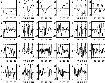
Several different structures for the model were tested. The number of source signals and the number of Gaussians in the mixtures was varied. The number of Gaussians in the mixtures was same for all sources in each network. This is not to say that it would not be perfectly simple to optimise the number of Gaussians for each source separately.

It turned out that the Kullback-Leibler information was minimised by a network with 23 dimensional source signals whose distributions were mixtures of three Gaussians. There were 87 292 unknown variables in the model: 86 227 in s(t); 782 in A; 68 in b and $\sigma$; 207 in c, S and $\gamma$; and 8 in hyperparameters.

  

Figure 1: Each row vector of $\hat{A}$ is a 34 dimensional basis vector corresponding to one source. The frequency increaces from left to right in all the subimages.

  

Figure 2: The histograms of the means $\hat{s}_i(t)$ of the sources.

  

Figure 3: The distributions of the sources reconstructed from $\hat{c}$, $\hat{S}$ and $\hat{\gamma}$.

Figures 1-3 show the basis vectors, histograms and reconstructed distributions of the 23 source signals of the best network. The ordering in all three figures is the same. The basis vectors in figure 1 probably do not seem very interesting for someone who is not working with speech recognition. The basis is fairly close to cosine transformation which is widely used for processing the spectra in speech recognition.

The histograms in figure 2 and the corresponding distributions in figure 3 show that the algorithm works. The model has captures the salient features of the source distributions, some of which are multimodal, skewed or kurtotic.

The second best fit was obtained by a network with two Gaussian in the mixtures, but the probability mass it captured was over 10⁷⁶ times smaller! It is therefore reasonable to approximate the whole posterior pdf of all model structures and parameters by an ensemble with a peak in only one model structure. It is also evident that in this case, any prior information about the model structure has no significance.

For comparison, also models with only one Gaussian in the mixtures were tested. In this case the logarithmic mixture coefficients c_ij can be dropped out from the model. The best model with only one Gaussian was found to have over 10¹²³⁸ times less probability mass. This shows that the algorithm agrees with human eye: it is clear that the distributions of at least some of the source signals are far from Gaussian.