Terms of the Cost Function

Almost all the distributions appearing in our model are assumed to be Gaussians, and consequently almost all the terms appearing in the cost function are expectations of logarithms of Gaussian distributions. We shall use the second layer biases a as an example. For each element a_i, there is one term in $q(\boldsymbol{\theta})$ and $p(X, \boldsymbol{\theta})$, namely the terms q(a_i) and p(a_i | m_a, v_a). The cost function therefore includes terms $\int q(\boldsymbol{\theta}) \ln q(a_i) d\boldsymbol{\theta}$ and $-\int q(\boldsymbol{\theta}) \ln p(a_i \vert m_a, v_a) d\boldsymbol{\theta}$. In the first expectation the terms q(a_i)only depends on a_i which means that we can integrate over the other variables and we have

$$\int q(\boldsymbol{\theta}) \ln q(a_i) d\boldsymbol{\theta} = \int q(a_i) \ln q(a_i) da_i \, .$$ (17)

The same happens for the other integral:
 $$\begin{multline}- \int q(\boldsymbol{\theta}) \ln p(a_i \vert m_a, v_a) d\boldsy... ... q(a_i)q(m_a)q(v_a) \ln p(a_i \vert m_a, v_a) da_i dm_a dv_a \, . \end{multline}$$
Recall that q(a_i) is Gaussian with mean $\bar{a}_i$ and variance $\tilde{a}_i$. This means that the integral in (17) yields simply

$$\int q(a_i) \ln q(a_i) da_i = -\frac{1}{2}\ln 2\pi e \tilde{a}_i \, .$$ (18)

The integral in (18) also fairly easy and it can be shown that the result is
 $$\begin{multline}- \int q(a_i)q(m_a)q(v_a) \ln p(a_i \vert m_a, v_a) da_i dm_a dv... ...tilde{v}_a - 2\bar{v}_a) + \bar{v}_a + \frac{1}{2} \ln 2 \pi \, . \end{multline}$$
Again the result is based on the fact that q(a_i), q(m_a) and q(v_a) are Gaussian with means $\bar{a}_i$, $\bar{m}_a$, $\bar{v}_a$and variances $\tilde{a}_i$, $\tilde{m}_a$, $\tilde{v}_a$, respectively.

The following terms are the only ones whose expectations in (16) give different results than (19) or (20): q(M_i(t), s_i(t)), p(M_i(t) | c_i), p(s_i(t) | M_i(t), m_si, v_si) and $p(x_k(t) \vert \boldsymbol{\theta})$.

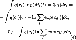
The index M_i(t) is discrete and therefore we have a summation instead of integration in the cost function. Let us denote $\dot{s}_{il}(t) = Q(M_i(t) = l)$ and denote the mean and variance of the Gaussian q(s_i(t) | M_i(t) = l) by $\bar{s}_{il}(t)$ and $\tilde{s}_{il}(t)$. Then the expectations of $\ln q(M_i(t), s_i(t))$ in (16) are given by
$$\begin{multline}\sum_l \int q(\boldsymbol{\theta}) \ln q(M_i(t) = l, s_i(t)) d\... ...dot{s}_{il}(t) - \frac{1}{2} \ln 2 \pi e \tilde{s}_{il}(t)] \, . \end{multline}$$
For the expectation of $-\ln p(M_i(t) \vert \mathbf{c}_i)$ we shall first evaluate the following integral:
$$\begin{multline}-\int q(\mathbf{c}_i) \ln p(M_i(t) = l\vert \mathbf{c}_i)d\mathb... ...+ \int q(\mathbf{c}_i) \ln \sum_{l'} \exp(c_{il'}) d\mathbf{c}_i \end{multline}$$
The resulting integral can be approximated by applying a second order Taylor's series expansion of $\ln \sum_{l'} \exp(c_{il'})$ with respect to c_il' around the posterior mean $\bar{c}_{il'}$. This yields the following approximation for the integral:
$$\begin{multline}-\int q(\mathbf{c}_i) \ln p(M_i(t) = l\vert \mathbf{c}_i)d\mathb... ...1}{2} \sum_{l'} \phi_{il'} (1 - \phi_{il'}) \tilde{c}_{il'} \, , \end{multline}$$
where $\phi_{il} = \exp(\bar{c}_{il}) / \sum_{l'} \exp(\bar{c}_{il'})$. Now we see that the expectation of $-\ln p(M_i(t) \vert \mathbf{c}_i)$ is
$$\begin{multline}-\sum_j \dot{s}_{il} \int q(\mathbf{c}_i) \ln p(M_i(t) \vert \ma... ...c{1}{2}\sum_{l'} \phi_{il'} (1 - \phi_{il'}) \tilde{c}_{il'} \, . \end{multline}$$
Since both q(s_i(t) | M_i(t)) and p(s_i(t) | M_i(t), m_si, v_si) are Gaussian, the terms $-\ln p(s_i(t) \vert M_i(t), \mathbf{m}_{si}, \mathbf{v}_{si})$ have expectations which are similar to (20):
$$\begin{multline}-\sum_l \dot{s}_{il} \int q(s_i(t) \vert M_i(t) = l) q(m_{sil}) ... ...ert M_i(t) = l, m_{sil}, v_{sil}) ds_i(t) dm_{sil} dv_{sil} \, , \end{multline}$$
which equals to the sum of terms
$$\begin{multline}\frac{1}{2}[(\bar{s}_{il}(t) - \bar{m}_{sil})^2 + \tilde{s}_{il}... ...il} - 2\bar{v}_{sil}) + \\ \bar{v}_{sil} + \frac{1}{2} \ln 2 \pi \end{multline}$$
weighted by $\dot{s}_{il}$.

The observations x_k(t) are known -- unless there are missing values -- which means that there are no terms of the form $\ln q(x_k(t))$. The expectations of $-\ln p(x_k(t) \vert \boldsymbol{\theta})$ are the most difficult terms in the cost function. If the posterior mean and variance of the function f_k(s(t)) are known -- let us denote them by $\bar{f}_k(t)$ and $\tilde{f}_k(t)$ for short -- then the expectation has a form similar to (20):
 $$\begin{multline}\frac{1}{2}[(x_k(t) - \bar{f}_k(t))^2 + \tilde{f}_k(t)] \exp(2\... ... - 2\bar{v}_{nk}) + \\ \bar{v}_{nk} + \frac{1}{2} \ln 2 \pi \, . \end{multline}$$