The result of learning is an approximation of the posterior probability of all the unknown variables given the observations. The unknown variables are the factors s(t), the parameters of the mapping f, variance parameters for factors and observation noise and the parameters of the hierarchical prior. The approximation is needed because the posterior joint probability of all the unknown variables is very complex due to the large number of unknowns and the complex structure of the model.
In most publications of this thesis, the approximation of the posterior is assumed to have a maximally factorial form, that is, all the unknown variables are assumed to be independent given the observations. This can be seen as a necessary and sufficient extension to point estimates which is sensitive to posterior probability mass instead of probability density. Publication VIII shows how some of the most important posterior correlations of the variables can be included in the approximation without compromising the computational efficiency. Notice that although the variables are assumed to be independent a priori, they are dependent a posteriori because the observations induce dependences between them.
Publication I presents the methods in minimum message length framework and therefore uses a uniform distribution as the approximation for the posterior. Other publications use the Gaussian distribution which is in general a better approximation to posterior densities. It is also often possible to choose a parameterisation, such as the logarithmic parameterisation of the variance or the ``softmax'' parametrisation of the mixture coefficients [84], which makes the Gaussian approximation even more valid.
The cost function in ensemble learning is the Kullback-Leibler information between the posterior probability and its approximation. Due to the simple factorial form of the approximation, the cost function and its derivatives can be computed efficiently. The required computations resemble very much the ones which would be carried out using the standard backpropagation algorithm for estimating the unknown variables of the model. The most notable difference is that scalar values are replaced by probability distributions of the values.
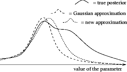
During learning, the approximation of the posterior is adapted by a modification of gradient descent which utilises the structure of the problem as explained in publication V. The difference to ordinary point estimation is that the weights and factors are characterised by their mean and variance. This is important as then the algorithm is sensitive to the probability mass in the posterior probability instead of being sensitive to probability density. Figure 7 illustrates the adaptation of the posterior probability density instead of a point estimate for an unknown variable of the model.
 |