Multilayer perceptrons

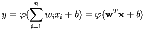
An MLP is a network of simple neurons called perceptrons. The basic concept of a single perceptron was introduced by Rosenblatt in 1958. The perceptron computes a single output from multiple real-valued inputs by forming a linear combination according to its input weights and then possibly putting the output through some nonlinear activation function. Mathematically this can be written as

$$y = \varphi( \sum\limits_{i=1}^n w_i x_i + b ) = \varphi( \mathbf{w}^T \mathbf{x}+ b )$$ (4.14)

where $\mathbf{w}$ denotes the vector of weights, $\mathbf{x}$ is the vector of inputs, $b$ is the bias and $\varphi$ is the activation function. A signal-flow graph of this operation is shown in Figure 4.1 [21,5].

The original Rosenblatt's perceptron used a Heaviside step function as the activation function $\varphi$. Nowadays, and especially in multilayer networks, the activation function is often chosen to be the logistic sigmoid $1 / (1 + e^{-x})$ or the hyperbolic tangent $\tanh(x)$. They are related by $(\tanh(x) + 1)/2 = 1 / (1 + e^{-2x})$. These functions are used because they are mathematically convenient and are close to linear near origin while saturating rather quickly when getting away from the origin. This allows MLP networks to model well both strongly and mildly nonlinear mappings.

Figure 4.1: Signal-flow graph of the perceptron

A single perceptron is not very useful because of its limited mapping ability. No matter what activation function is used, the perceptron is only able to represent an oriented ridge-like function. The perceptrons can, however, be used as building blocks of a larger, much more practical structure. A typical multilayer perceptron (MLP) network consists of a set of source nodes forming the input layer, one or more hidden layers of computation nodes, and an output layer of nodes. The input signal propagates through the network layer-by-layer. The signal-flow of such a network with one hidden layer is shown in Figure 4.2 [21].

The computations performed by such a feedforward network with a single hidden layer with nonlinear activation functions and a linear output layer can be written mathematically as

$$\mathbf{x}= \mathbf{f}(\mathbf{s}) = \mathbf{B}\boldsymbol{\varphi}( \mathbf{A}\mathbf{s}+ \mathbf{a} ) + \mathbf{b}$$ (4.15)

where $\mathbf{s}$ is a vector of inputs and $\mathbf{x}$ a vector of outputs. $\mathbf{A}$ is the matrix of weights of the first layer, $\mathbf{a}$ is the bias vector of the first layer. $\mathbf{B}$ and $\mathbf{b}$ are, respectively, the weight matrix and the bias vector of the second layer. The function $\boldsymbol{\varphi}$ denotes an elementwise nonlinearity. The generalisation of the model to more hidden layers is obvious.

Figure 4.2: Signal-flow graph of an MLP

While single-layer networks composed of parallel perceptrons are rather limited in what kind of mappings they can represent, the power of an MLP network with only one hidden layer is surprisingly large. As Hornik et al. and Funahashi showed in 1989 [26,15], such networks, like the one in Equation (4.15), are capable of approximating any continuous function $\mathbf{f}: \mathbb{R}^n \rightarrow \mathbb{R}^m$ to any given accuracy, provided that sufficiently many hidden units are available.

MLP networks are typically used in supervised learning problems. This means that there is a training set of input-output pairs and the network must learn to model the dependency between them. The training here means adapting all the weights and biases ( $\mathbf{A}, \mathbf{B}, \mathbf{a}$ and $\mathbf{b}$ in Equation (4.15)) to their optimal values for the given pairs $(\mathbf{s}(t), \mathbf{x}(t))$. The criterion to be optimised is typically the squared reconstruction error $\sum_t \vert\vert\mathbf{f}(\mathbf{s}(t)) - \mathbf{x}(t)\vert\vert^2$.

The supervised learning problem of the MLP can be solved with the back-propagation algorithm. The algorithm consists of two steps. In the forward pass, the predicted outputs corresponding to the given inputs are evaluated as in Equation (4.15). In the backward pass, partial derivatives of the cost function with respect to the different parameters are propagated back through the network. The chain rule of differentiation gives very similar computational rules for the backward pass as the ones in the forward pass. The network weights can then be adapted using any gradient-based optimisation algorithm. The whole process is iterated until the weights have converged [21].

The MLP network can also be used for unsupervised learning by using the so called auto-associative structure. This is done by setting the same values for both the inputs and the outputs of the network. The extracted sources emerge from the values of the hidden neurons [24]. This approach is computationally rather intensive. The MLP network has to have at least three hidden layers for any reasonable representation and training such a network is a time consuming process.