Point estimates

Point estimates use a single representative value to summarise the whole posterior distribution. The maximum likelihood (ML) estimate (or solution) for the unknown variables $\boldsymbol{\Theta}$ is the point in which the likelihood $p(\boldsymbol{X}\mid \boldsymbol{\Theta},\mathcal{H})$ is highest. The maximum a posteriori (MAP) estimate is the one with highest posterior probability density $p(\boldsymbol{\Theta}\mid \boldsymbol{X},\mathcal{H})$. Note that a common and even simpler criterion, the mean square error, is equivalent to the ML estimate assuming Gaussian noise with constant variance (Bishop, 1995).

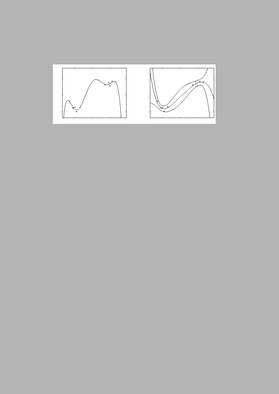
An iterative learning algorithm is said to overlearn the training data set, when its performance with unseen test data starts to get worse during the learning with training data (Chen, 1990; Haykin, 1999; Bishop, 1995). The system starts to lose its ability to generalise. The same can happen when increasing the complexity of the model. The model is said to overfit to the data. In this case the model becomes too complicated and concentrates on random fluctuations in the data. The left subfigure of Figure 2.2 shows an example of overfitting.

Figure 2.2: A sixth order polynomial is fitted to 10 data points. Left: Maximum likelihood solution. Right: Bayesian solution. The three curves present 5%, 50% and 95% fractiles.

When the model is too simple or the learning is stopped too early, the problem is called underfitting or underlearning respectively. Balancing between over- and underfitting has perhaps been the main difficulty in model building. There are several ways to fight overfitting and overlearning (Chen, 1990; Haykin, 1999; Bishop, 1995). A popular method is to select the best time to stop learning or the best complexity of a model by cross-validation (Stone, 1974; Haykin, 1999). Part of the training data is left for validation and the models are compared based on their performance with the validation set.

The problems of overlearning and overfitting are mostly related to point estimates. The example in Figure 2.2 is solved by using the whole posterior distribution instead of a single solution. The use of a point estimate is to approximate integrals so it should be sensitive to the probability mass rather than to the probability density. Unfortunately, ML and MAP estimates are attracted to high but sometimes narrow peaks. Figure 2.3 shows a situation, where search for the MAP solution first finds a good representative of the probability mass, but then moves to the highest peak which is on the border. This type of situation seems to be very common and the effect becomes stronger, when the dimensionality increases. Appendix D of Publication I gives an example where point estimates fail completely.

Figure 2.3: A hypothetical posterior pdf. A point estimate could first find a good representative of the probability mass, but then overfits to a narrow peak.