The Bayesian probability theory and decision theory sound too good to be true: They solve learning, inference, and decision making optimally. Unfortunately, the posterior probability distribution cannot be handled analytically except in the simplest examples. To solve the integrals in Equations (2.2), (2.3), and (2.4), one must resort to some kind of approximations. There are three common classes of approximations: point estimates, sampling, and variational approximations.
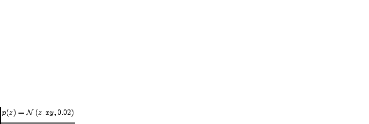
Figure 2.1 shows two posterior distributions. The models are not particularly meaningful (having just two unknown variables), but they are chosen to highlight differences in various posterior approximations, which are described in the following.
![\includegraphics[width=0.44\textwidth]{posterior1.eps}](img94.png)
![\includegraphics[width=0.45\textwidth]{posterior2c.eps}](img95.png)
|
 and
and  are shown in black
contours. Maximum a posterior estimate is plotted as a red star,
Bayes estimate (or the expectation over the posterior) is plotted as a red circle. Variational Bayesian
solution with a Gaussian posterior approximation with diagonal
covariance is shown in blue as a dot surrounded by ellipses. Left: model
are shown in black
contours. Maximum a posterior estimate is plotted as a red star,
Bayes estimate (or the expectation over the posterior) is plotted as a red circle. Variational Bayesian
solution with a Gaussian posterior approximation with diagonal
covariance is shown in blue as a dot surrounded by ellipses. Left: model
 ,
observation
,
observation  , priors
 ,
,
 . Right: model
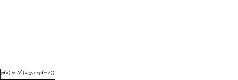 ,
observation
,
observation  , priors
 ,
,
 .
.