Performance with the speech data

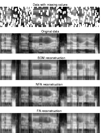
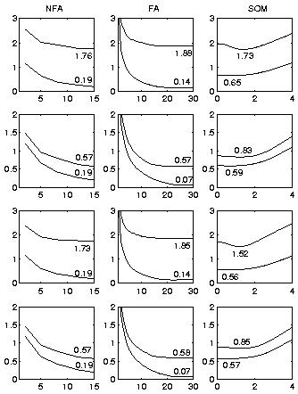
The performance of different methods with speech data can be seen in Figure 5. NFA was tested with 30 hidden neurons and 2 to 15 factors and FA with number of factors varying from 1 to 30. The implemented NFA algorithm suffered from instability when the number of factors was greater than 15. The NFA model performed always better than FA with same number of factors.

The mean square reconstruction errors are collected here in the same order as in Figure 3:

NFA			FA			SOM
1.76	0.57		1.88	0.57		1.73	0.83
1.73	0.57		1.85	0.58		1.52	0.85

The first setting proved to be the hardest as expected, since new words require generalisation and missing values in patches makes nonlinear effects more important. With optimal parameter values the SOM gave marginally better reconstructions than NFA. FA performed the worst.

The second setting was easier: NFA and FA performed equally well, but the SOM could not achieve same accuracy. A large number of model vectors did not help the SOM to get enough representing power.

The third setting had permuted data sets, which makes generalisation less important. This helped the SOM a lot and it gave clearly the best results. NFA and FA benefitted only marginally and were left behind.

Results of the fourth setting did not differ from the second setting. The change in the missing value pattern from the first and third settings seems to have the dominant effect.

The reconstruction errors of the observed values (lower curves in Figure 5) are of interest, too. The SOM cannot represent the data as accurately with the map unit activities as the factor analysis models can with the factor values. The FA model with 30 factors could have represented the data perfectly, but the modelled noise accounted for some variation.

The best number of model vectors in the SOM was 1600 in the first case, but at least 2400 in the other cases. This has caused a change in the reconstruction error of the observed values. The optimal width of the softening kernel was also somewhat larger in the first experiment. The number of map units is normally not as large as half of the number of data vectors.

  

Figure 4: Speech data reconstruction example with best parameters of each algorithm.

  

Figure 5: Mean square reconstruction errors of speech data as a function of number of factors or softening width. The rows correspond to the experiment settings reading from up to down. The upper curve in each plot is the test result for missing values and the lower curve is the reconstruction of observed values.