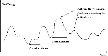
Figure: Energy (vertical axis) defined for a one-dimensional state space.
Some of the algorithmic approaches mentioned above will be described here, including those that were experimentally applied and studied in practice in this work (see next section).
One way to solve a problem is to describe it in terms of a graph with nodes as states in the problem-solving process and edges as transitions between states, i.e. steps to take in search of a good solution. There exists a multitude of different graph-searching techniques from elementary brute-force methods such as depth-first and breadth-first to rather exclusive ones such as tabu search. We will discuss only one of these here, the heuristic graph search.
Heuristics are rules of thumb that guide the search of good solutions to a problem. In graph searches heuristics are used to select the most promising-looking branch of the search tree or graph. These branches may then be examined first, before others, or even to cut out parts of the search tree altogether.
Good heuristics can reduce the time required to find a good-enough solution, compared to brute-force methods. However, with bad heuristics, finding the solutions may take very long. If the heuristics are bad enough, they may guide to bad solutions instead of good ones. Thus, the heuristic algorithm may perform even worse on the average in terms of time used to find an acceptable solution than a brute-force search without heuristics. Even worse, the acceptable solutions may not be found at all, if the heuristics are used to cut out branches of the search tree without examining them.
The problem with heuristics is how to decide half-way what would be an appropriate next action, i.e. how to design heuristic rules that lead to good solutions instead of bad ones. The following are only a few examples of possible heuristics that could be used to guide a search for good layout configurations:
The third type of layout problems (fixed free area, variable content) may be approached as bin-packing problems. The basic bin-packing problem, as described in [Hofri, 1987], consists of an unlimited (or large) number of bins of equal size and of a number of items of variable sizes. The task is to fit the items into the bins so that a minimum number of bins is used and the capacity of no bin is exeeded. Some pagination problems fit this formulation approximately: Each page is represented as a bin, and the given material is represented as the items to be packed.
There are many algorithms for solving bin-packing problems in one dimension, although the problem is NP-hard in the strong sense. However, as the dimension grows the problem quickly becomes very complex. Even the 2-dimensional case is rather difficult to solve. Furthermore, many pagination problems involve different kinds of constraints (see section 3.1 for examples in newspaper pagination) that would need to be integrated into the pure bin-packing algorithms.
Genetic algorithms (GA) have been applied to latter two of the above described three problem types. The major difficulties, as reported by [Hwang et al., 1994] have been encountered in developing a representation of the bin-packing problem that is suitable for a GA and is not limited to cuttings representable by slicing trees. The same authors also reported using GA's successfully for improvement of the solutions found by heuristic algorithms, and suggested combining simulated annealing with genetic algorithms.
Simulated annealing (SA) is a stochastic optimization method that may be used to minimize a given cost function (energy), given a possibly combinatorial system with many degrees of freedom. The algorithm has been described in numerous publications, including the seminal paper [Kirkpatrick et al., 1983], and a book [Aarts and Korst, 1989] containing a thorough analysis of the theory and its relation to Markov Theory, and applications. A concise overview of the SA may be found e.g. in [Haykin, 1994]. When not otherwise stated, the following description of SA is in accordance with [Haykin, 1994].
The idea for SA is drawn from statistical physics, especially from the theory of cooling solids. According to the theory, if a substance is cooled slowly enough from a sufficiently high starting temperature (melting point), it will arrange itself into a low-energy lattice structure. If the cooling is too rapid, the system will freeze into a non-optimal state, with "errors", i.e. unsymmetries, in the lattice structure.
The annealing metaphor can be changed into an optimization algorithm as follows:
In this algorithm, "temperature" translates to a probabilistic parameter defining how often deteriorating changes are accepted, and "cooling" into reducing the probability. A solution to the problem corresponds to the state of a physical system, and the cost of the solution to the energy of the state. Thus, optimal solutions (and faultless crystals) are represented by the global minima of the cost or energy landscape (see Fig. 2).

Figure: Energy (vertical axis) defined for a one-dimensional
state space.
The changes are accepted according to the following function:

where T is analogous to temperature and E refers to energy of the
state. After enough rounds in a temperature, the system will reach a
thermal equilibrium in which the probability of being in a state
depends on the energy of the state, i.e.  is a function of
 , the Boltzmann distribution, for the given temperature
T. When the system has reached the thermal equilibrium, the
temperature may be decreased.
Thus, at high temperatures (i.e. in the beginning of the simulation), changes are mostly accepted regardless of whether they are improvements or not. As the temperature slowly drops, the big up-hill changes are increasingly rejected. Finally, in zero temperature SA behaves like a normal gradient-descent search technique where only downhill changes (i.e. immediate improvement in the system state, measured by the energy function) are accepted.
To understand why this method works, the following intuitive explanation may help: When temperature is high, there is enough thermal noise in the system to climb over high hills of the energy landscape (see again Fig. 2). With low temperatures, the thermal noise is lesser and high hills are rarely climbed over. Finally, with zero temperature, the state has no "internal energy" to climb over high hills and only downhill changes are possible. At this point the system soon freezes into one state or oscillates between states with equally low energy.
The following steps must be taken when implementing this algorithm for a given optimization problem [Haykin, 1994]:
To sensibly apply SA, the state space must be defined so that there is some kind of topology, and so that the connectivity between states, defined by the state transitions, is not complete. It is evident why the connectivity should not be complete: with complete connectivity there is a path of length one from any node to any other node. In this situation full search performs better than SA. This fact becomes evident even without a mathematical proof from the following analogy: The state space is represented by an apple basket and each state by an apple. With each step, one apple is selected from the basket. In deterministic, full search, the apple is taken out from the basket and measured, and not returned. The best apple is always kept aside. Each apple is encountered exactly once. In SA, the apple is returned to the basket after measurement, and may subsequently be retrieved and measured many times, because of the symmetry of the states. SA has no memory of what apples (states) were already measured.
The need for "sufficient" connectivity is also intuitively rather clear: if the connectivity is minimal, in the worst case the state space is a linked list of states. Again, deterministic search, i.e. going through the states in the list order, performs clearly better than SA. This is because for SA to work according to the theory, each temperature should be kept long enough so that an equal probability distribution of being in any state is achieved in that temperature. With a list, approaching the equal probability distribution is extremely slow.
SA apparently works best in a situation where there are areas of the state space with several "rather good" solutions rather close to each other (i.e. with topology). This way, by sampling the space the system may proceed to areas with more good samples (this is achieved by approximately reaching the thermal equilibrium) and look at them closer, i.e. in a lower temperature.
SA differs from gradient-descent optimization procedures in that it
does not necessarily get stuck in a local minimum. The SA method, if
applied by the theory, i.e. if annealing is performed slowly enough,
is guaranteed to find the globally optimal solution. According to
Geman and Geman (1984) as cited in [Haykin, 1994], with sufficiently
large  , if the following applies for every k,

the system will converge to miminum energy configuration with probability one. Unfortunately, this cooling schedule is too slow to be used in any practical system. However, practical approximations of the schedule often produce near-optimal solutions to the given problem, especially when there are many such solutions.
Simulated annealing has previously been applied to minimization of layout area and wire length on VLSI layout design [Sugai and Hirata, 1991], and to machine layout problems in manufacturing where transportation of production resources between different machines must be minimized [Kouvelis et al., 1992].