Fast Variational Bayesian Linear State-Space Model

Fast Variational Bayesian Linear State-Space Model

Jaakko Luttinen, ECML/PKDD, 2013
The final publication is available at link.springer.com
[Paper PDF] (author-created version, permitted by Springer publication, fixed errors in (21) and (22))
[Poster PDF]
[Slides PDF]

ERRATA: The equations (21) and (22) contain typos in the published version. The correct formulas are in the author-created version.

The paper presented a fast variational Bayesian method for linear state-space models. The standard variational Bayesian expectation-maximization (VB-EM) algorithm is improved by a parameter expansion which optimizes the rotation of the latent space. With this approach, the inference is orders of magnitude faster than the standard method. A Python implementation of the method, the data and the experiment scripts are distributed under open licenses below. The instructions are written for Linux users but may be applicable to Windows users if modified appropriately.

BayesPy - Bayesian Python

The parameter expansion is implemented in BayesPy package, a new Python package for variational Bayesian inference, and it is available under the GNU GPLv3 license. It can be installed from PyPI or GitHub.

Installing the requirements

BayesPy requires Python 3.2 and a few Python packages: NumPy (>=1.7.1), SciPy (>=0.11), matplotlib (>=1.2), Cython and h5py. The installation of those packages is out of the scope of these instructions, thus you may refer to the official SciPy installation instructions. At least NumPy and Cython must be installed before installing BayesPy. The other required packages are installed automatically when installing BayesPy but that might not work unless you have installed a C compiler, Python development files, BLAS/LAPACK libraries and some other system dependencies. Please refer to the documentation of BayesPy for more detailed instructions on the installation of the requirements. In any case, this is just a matter of installing five popular packages for Python 3.2, so it should be quite straightforward and the web should contain lots of instructions. It is recommended that you install BayesPy and the requirements under virtualenv but that is not necessary. To create and activate a new virtual environment, run

virtualenv -p python3.2 --system-site-packages ENV
source ENV/bin/activate

The virtual environment is stored in the folder ENV.

Installing BayesPy

After the requirements have been installed, BayesPy can be installed simply as

pip install bayespy

The source code of BayesPy is available at GitHub. General documentation of the package is available at bayespy.org. In particular, the documentation contains a section discussing the linear state-space model and the rotations as presented in the paper.

Running the experiments

The scripts for running the experiments in the paper using BayesPy are also available:
Download the Python scripts for the experiments.
After unpacking, a simple help text can be printed using:

python run_experiment.py --help

For instance, the artificial experiment can be run using the following commands


python run_experiment.py --experiment=small --maxiter=10000
python run_experiment.py --experiment=small --maxiter=10000 --rotate

and the Testbed experiment using the following commands


python run_experiment.py --experiment=testbed --maxiter=1000
python run_experiment.py --experiment=testbed --maxiter=1000 --rotate

Note that the Testbed experiment requires that the Testbed dataset (available below) is in the same folder and that running the experiments may take a very long time. The experiments save the VB results automatically after every 10 iterations and those results can be opened for closer examination. These results can be used for a similar comparison as was shown in the paper by using a plotting script:

python plot_experiment.py --baseline="results/your_baseline_file.hdf5" --rotations="results/your_rotations_file.hdf5"

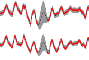
If you do not see any figure, your matplotlib is probably misconfigured. Note that you may need to zoom in to see the speed-up effect well. The results can be examined in more detail in the Python environment by loading the results and then using NumPy/BayesPy tools. For instance, the predictive/reconstruction distribution of the observed process can be plotted as

import matplotlib.pyplot as plt
import bayespy.plot.plotting as bpplt
import numpy as np
import run_experiment
# Load the results
Q = run_experiment.load_results(filename)
# Compute the predictive distribution
(mean_y, var_y) = Q['Y'].predict()
# Plot the timeseries predictions
plt.ion()
bpplt._timeseries_mean_and_std(mean_y, np.sqrt(var_y), axis=-1)

Future experiments could include, for instance, higher dimensional latent space for the Testbed experiment (using --D option) and different datasets.

Helsinki Testbed data

Download the dataset in HDF5 form.
The producer of the dataset and the holder of database rights is the Helsinki Testbed project.
The dataset is distributed under the Finnish Meteorological Institute's Open Data License.
The dataset contains temperature measurements from Southern Finland over the period of 10/2005-06/2007. The temperature is measured at 10-minute interval in 198 locations (many of the locations are different altitudes at same weather stations). The full dataset contains 89202 time instances. It contains a large amount of missing values, badly corrupted measurements and some incorrect weather station coordinates. The dataset HDF5 file contains a matrix of measurements (rows corresponding to stations and columns corresponding to time instances), the coordinates of the stations and the timestamps (proleptic Gregorian ordinal, where 1 January 1 has ordinal 1).

Extra material: Gradients

The optimization of the rotation requires the gradients with respect to the rotation matrix. These were left out from the paper in order to keep the paper concise, but they are provided here as extra material available as PDF (or raw LaTeX).