Prediction accuracy

An obvious way to assess the quality of the learned model is to see on how long term the predictions given by the model are accurate. It should be noted that since the Lorenz process is chaotic, it is numerically impossible to predict it exactly in the distant future. The best that can be hoped for is to capture the overall aspects of the long-term behaviour. Figure 6 confirms that this is accomplished by the NDFA algorithm.

  

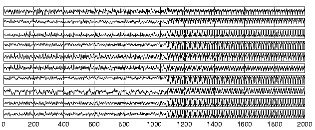
Figure 7: The ten plots show the original observations x(t) $(1 \leq t \leq 1000)$ and the result of prediction made by a nonlinear auto-regressive model $(t \geq 1001)$. The noise process was omitted like in the results shown in figures 5 and 6.

For comparison, the prediction of the future observations was tested with a nonlinear auto-regressive (NAR) model

$${\mathbf{x}}(t) = {\mathbf{h}}({\mathbf{x}}(t-1), {\mathbf{x}}(t-2), \ldots, {\mathbf{x}}(t-D)) + {\mathbf{n}}(t) \, .$$ (19)

Several strategies were tested and the best performance was given by an MLP network with 20 inputs and one hidden layer of 30 neurons. The inputs to the MLP network were the principal components extracted from the sequence of ten past observations, that is, D was ten. Figure 7 shows the performance of this NAR model. It is evident that the prediction of new observations is a challenging problem. Principal component analysis used in the model can extract features which are useful in predicting the future observations but clearly the features are not good enough for modelling the long-term behaviour of the observations.

  

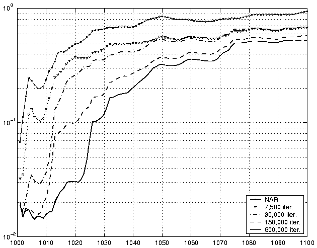
Figure 8: The average cumulative squared prediction error is computed for the predictions made using the NDFA algorithm after 7500 (dotted with triangles), 30,000 (dash-dotted), 150,000 (dashed) and and 600,000 iterations (solid) as well as by a nonlinear auto-regressive model (solid with dots). The predictions are based on 100 Monte-Carlo simulations of the estimated dynamics. Taking into consideration the observation noise whose variance is 0.01, the prediction obtained by the NDFA algorithm in the end of learning is excellent up to t = 1010 and fairly good up to t = 1022. The NAR model is quite inaccurate already after $t \geq 1003$.

Both the NAR model and the model used in NDFA algorithm contain noise process which can be taken into account in the prediction by Monte-Carlo simulation. Figure 8 shows the results obtained by 100 runs of Monte-Carlo simulation. The average predicted observations are compared to the actual continuation of the process. The figure shows the average cumulative squared prediction error. Since the variance of the noise on the observations is 0.01, the results can be considered perfect if the average squared prediction error is 0.01. The signal variance is 1, which gives the practical upper bound of the prediction accuracy. The figure confirms that the NDFA algorithm has been able to model the dynamics of the process as the short-term average prediction error is close to the noise variance. Even the long-term prediction falls below the signal variance which indicates that at least some part of the process can be predicted in the more distant future. The steady progress made during learning is also evident.

  

Figure 9: The factors s(t) have been predicted by Monte-Carlo simulations. The mean $\mu$ (dashed) and range $\mu \pm \sigma$ (solid) obtained from the simulation runs are shown.

  

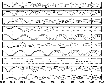Figure 10: The factors in figure 9 are mapped on the original state space. The mean (dotted) and range (dashed) together with the true continuation (solid) are shown. Due to the chaotic nature of the Lorenz system, the state cannot be predicted for distant future. Notice, however, how the model has been able to predict the timing of the oscillations for the first and fourth states although the sign is uncertain.

  

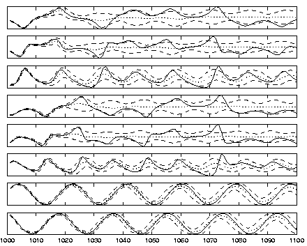Figure 11: The factors in figure 9 are projected onto the observations by the estimated mapping f. The mean (dotted) and range (dashed) together with the true continuation (solid) are shown.

  

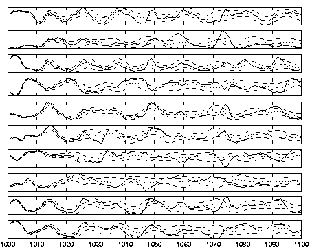Figure 12: Monte-Carlo simulations with the NAR model have been used for predicting the observations. The mean (dotted) and range (dashed) together with the true continuation (solid) are shown.

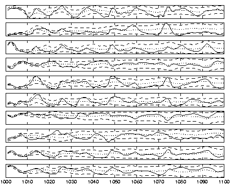Figures 9-12 show the results of the Monte-Carlo simulations for individual time series. Each plot shows the averages $\mu$ and the range $\mu \pm \sigma$ as obtained from the simulations. Here $\sigma$ stands for the standard deviation. Figure 9 depicts the predicted continuation of the factors s(t). In figure 10, these are mapped to the original state space while figures 11 and 12 show the predicted observations obtained by the NDFA algorithm and NAR model, respectively, together with the true continuation.