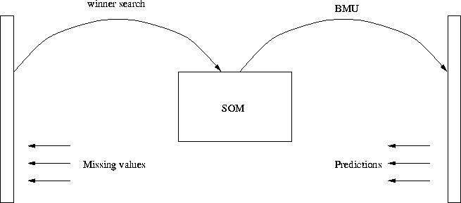
Figure 4.1: Fetch the unknown variables
The SOM is a nonparametric regression model. This provides a data-driven abstraction method of the phenomenon described by input data. It is possible to study the general case by building this kind of model from many individual cases.
The codebook vectors of the SOM represent the general form of the data and quantize the input space. Along with the training, the elastic net is streched to cover the cloud of data in the input space. We can use this representation as a model or build models on this abstraction. We can visualize the SOM by drawing a U-matrix or a component plane representation described earlier in section 2.2.4. These provide us information about the correlations between components, division of data in the input space and relative distributions of the components.
The problem of scale selection must be tackled. The scale selection is the problem of determining the smallest level of detail, or the granularity. This corresponds, in a plain SOM representation, to picking a suitable number of codebook vectors. Heuristics can be developed to do this, but this always requires that assumptions are made by the observer. Training a SOM with a large number of neurons requires a lot of computational effort and one may end up modeling small details. A SOM with a small number of neurons might not in turn grasp the essential.
Suppose we train a SOM with input vectors of dimension n. SOM is then a representation of the general case with no regard to which components of the input vector are independent variables and which are dependent variables. We have not committed us to a certain relationship between the vector components or named any components as the ``inputs'' or the ``outputs'' of this relationships.
We can constrain any component of the input vector to be constant and to fetch the rest of the vector values with the aid of known values. The forecasted values are then the values of the BMU with regard to the known values of the input vector.
The credibility measure of the predicted values can be approximated by the difference between the codebook vector and the input vector.

Figure 4.1: Fetch the unknown variables
A prediction can be created by seeking the best-matching unit for the a vector with unknown components with regard to the known components. The winner unit is searched with regard to the known components only. The predicted values can be fetched from the best-matching unit.
A same kind of approach was used in robot control by Ritter et al. [35]. The SOM was used as an adaptive look-up table for fetching suitable output variable values for given input variable values. Output values correspond to control actions with given input values. Output values were taught with a different learning rule. This corresponds to ``picking the most suitable question for our question, and finding the corresponding answer and considering that for a final answer''. Kohonen suggests that this might be the way brain operates, namely by fusing different kinds of data together [20]. In the second application in time series prediction by Walter et al. [42] the SOM was used to partition the state-space of a time-dependent system. Each state of the system was mapped to a codebook vector, and the next state was predicted by an autoregressive model of the previous values of the system. The autoregressive models were specific to a certain state-space.
This method is indeed very simple. It is not committed to any ``inputs'' or ``outputs'', but can be used to predict any wanted ``input-output'' relationship. It would be desirable that the number of known components would be larger than the number of unknown components.