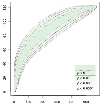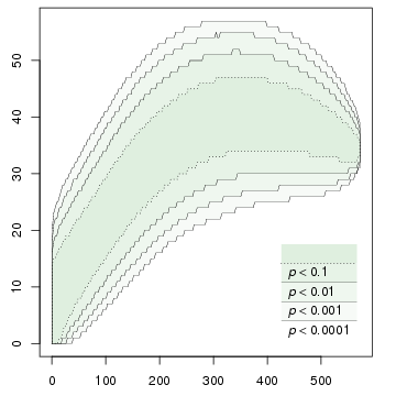

A program for computing accumulation curves of types and hapaxes. Uses permutation testing: constructs a number of random permutations of the input, and finds the upper and lower bounds for each significance level.
You can cite this software as follows:
News: A new, thoroughly revised version of this software is now available. Please note that the new version is not directly compatible with the data files used by the old version; some data conversion will be needed.


Given some samples of data where data items are classified into a number of types (classes), this program can be applied to test hypotheses which are related to type richness or the diversity of the data: whether there are relatively many or relatively few different types of items. Examples of such situations include the following:
The key concepts are best described by considering these concrete examples:
A sample can be described numerically by specifying the number of items of each type in the sample, as well as the total number of items in the sample.
Depending on the phenomenon that we are studying, we can label the samples with different attributes. In the case of texts, some samples may be labelled as being written by women; some samples may be labelled as being written by more educated people; some may be labelled as being written during the 17th century. In the case of animal species, some samples might be labelled as being collected in young forests, in coniferous forests, or in areas near human habitation.
Given a particular labelling of the samples, we are interested in testing the hypothesis that a particular labelling correlates with the number of types. For example, we want to know if the samples collected in young forests have a small number of different animal species; as a point of comparison we have any other set of samples with the same number of items.
More formally, let n be the number of items in the samples labelled with A. We use as the test statistic the number of types that are accumulated during the first n items. As a null hypothesis, we postulate that we can ignore the labels; the samples labelled with A are just chosen randomly from the set of all samples. In particular, the number of types in the samples labelled with A is not lower [not higher] than what is accumulated during the first n items in many random reorderings of the samples. However, if only a very small fraction of the reorderings has this property, we have to reject the null hypothesis and accept the alternative hypothesis that there are significantly few [many] types in the samples labelled with A. Note that we do not need to assume any specific parametric model; the only modelling assumption is that the ordering of the samples is exchangeable under the null hypothesis.
This program enables us to test such hypotheses efficiently. For a particular data set, the program needs to be executed only once; it tabulates upper and lower bounds on the number of types for different levels of significance and for various ranges of n. The figures at the beginning of this page are graphical illustrations of the output of the software; for example, if we are studying biodiversity, the curve on the left can be interpreted as a species accumulation curve with confidence intervals.
In addition to using the number of accumulated types as the test statistic, it is also possible to use the number of accumulated hapaxes (types with exactly one item) as the test statistic.
See the section “Usage” for a concrete example of applying the software, as well as for details on the interpretation of the results.
The program is written in standard C (ISO/IEC 9899:1999). It should compile and run on any standard-compliant platform. However, the Makefile distributed with the program and the following installation instructions are written for a modern GNU/Linux platform.
tar xzf types-2007-05-15.tar.gz
cd types-2007-05-15
make
make check
Copy the file “types” wherever you want and run it. No other files are needed.
Here is one possible way to install and run the program on Microsoft Windows. First, install MinGW. Open the command prompt and make sure that you can run the command “gcc”; a full path name such as “c:\mingw\bin\gcc” may be required. Switch to the directory in which the source file types.c is located, and compile it as follows:
gcc -g -O2 -std=iso9899:1999 -Wall -o types.exe types.c
This should produce the file types.exe. Copy the file wherever you want and run it. You can try the following command on the command prompt to run the program: “types --help”.
The program reads its input from the standard input stream. The input file consists of fields which are separated by whitespace (any number of spaces, tabulators and line feeds). A spreadsheet software with plain text output can be used to create the input file.
We use the file sample-input.txt as an example of an input file. The first two fields denote the number of samples (here 35) and the number of types (here 40):
35 40
The next fields give the name of each sample (here the samples are named with two-character labels aa, ab, etc.) and the number of items in the sample. Note that any kind of whitespace can be used to separate the fields, so you can add line feeds for clarity.
aa 113 ab 186 ac 162 ad  28 ae  77 af  37 ag  95 ah 147 ai  86 aj  44
ak  67 al  32 am  14 an  85 ao  93 ap 178 aq  92 ar  75 as 161 at  56
ba  41 bb  55 bc  65 bd  76 be  48 bf  85 bg  89 bh  40 bi  82 bj  16
bk  14 bl  89 bm  81 bn  64 bo 105
Next comes the name of each type. Here we have used the names t1, t2, etc.
t1  t2  t3  t4  t5  t6  t7  t8  t9  t10
t11 t12 t13 t14 t15 t16 t17 t18 t19 t20
t21 t22 t23 t24 t25 t26 t27 t28 t29 t30
t31 t32 t33 t34 t35 t36 t37 t38 t39 t40
Finally, we present the occurrences of the types in each sample. First, we give the occurrences of each type in the first sample. Here there were 0 occurrences of type t1, 1 occurrence of type t2, 0 occurrences of type t2, etc. in the first sample (aa).
Note that the sum of these figures does not have to equal the total number of items in the sample aa. In this example, the sum of these figures is 12 and the total number of the items was 113 (see above). For example, the types presented here may correspond to some specific words of interest, while there are also many other words in our text corpus.
0 1 0 0 1 0 0 0 0 0 0 0 0 0 0 0 0 2 0 0 0 0 0 0 1 0 0 1 0 2 1 1 0 1 0 1 0 0 0 0
Similarly, we give the number of types for the second sample, third sample, and so on (see the file sample-input.txt for all rows).
0 1 0 0 0 0 0 0 0 0 1 0 0 1 6 2 1 0 0 0 0 1 0 1 1 1 0 0 0 0 1 1 0 1 0 1 0 0 1 0
0 1 0 0 4 0 0 0 0 0 1 0 0 0 0 0 0 0 0 6 0 0 0 4 0 4 0 0 0 1 0 0 0 1 0 0 0 0 0 0
...
We are interested in studying the type richness in the samples b? (ba, bb, ..., bo). Put together, there are 26 different types and a total of 950 items in these samples. In the entire data set there are 40 different types and a total of 2778 items. Our hypothesis is that the samples b? are poor in type richness. Let us now test this hypothesis.
First, let us perform a quick test with 10 000 random samples at a resolution of 100 slots. We enter the following command (the switch --brief just omits some redundant rows from the output).
./types --brief 10000 100 < sample-input.txt
Running the program takes only a fraction of a second and prints the result to standard output. We can now quickly examine the output and see whether the results seem to be worth further investigation (see below for more information on interpreting the results). This seems to be the case and we run the program again with different parameters. 100 slots seems to be sufficient for our purposes; however, to make the probability of incorrect interpretation due to a biased sample negligible, we take 1 000 000 random samples:
./types --brief 1000000 100 < sample-input.txt > sample-output.txt
This time the program takes a bit longer to run (approx. 8 seconds on a desktop PC with a 2.4-GHz Pentium 4 processor). The result is stored in the file sample-output.txt
Let us now examine the file sample-output.txt. Here are selected parts of it:
       0    0    0    0    0    0   13   15   16   19   20
      28    0    0    0    0    0   15   17   20   23   26
      56    0    0    0    0    0   18   19   23   26   28
      84    0    0    0    0    0   20   22   25   28   30
     ...
     898   22   24   27   30   31   39   40   40   40   40
     926   23   25   28   30   32   39   40   40   40   40
     954   23   26   29   31   32   39   40   40   40   40
     982   24   26   29   31   33   39   40   40   40   40
     ...
    2610   39   40   40   40   40   40   40   40   40   40
    2694   39   40   40   40   40   40   40   40   40   40
    2722   40   40   40   40   40   40   40   40   40   40
    2778   40   40   40   40   40   40   40   40   40   40
The first column is the number of items. Because we specified on the command line that we wanted 100 slots of results, the results are computed for 100 different item counts. (Actually, there are slightly fewer lines than 100 because we gave the command line switch --brief; without it, the program would also print a line for, e.g., 2750 items; however, the results would be identical to the line immediately before it and the line immediately after it.)
The next 5 columns are lower bounds for the number of types at significance levels 0.0001, 0.001, 0.01, 0.05, and 0.1. The next 5 columns are upper bounds for the number of types at significance levels 0.1, 0.05, 0.01, 0.001, and 0.0001.
The b? samples had 26 different types and a total of 950 items. Let us now compare these figures to the above results which are constructed from all samples. We study the slots immediately surrounding the item count 950 in the table: the slot with 926 items and the slot with 954 items. We focus on the column which corresponds to the significance level of 0.01 (i.e., 1 %); there is the value 28 in slot 926 and the value 29 in slot 954. The output is conservative; we can choose the looser bound of the values 28 and 29. Therefore we obtain the following result:
The program sampled 1 000 000 random permutations; therefore it is not likely that this result is caused by an unfortunate choice of the random sample. Because 26 < 29, we conclude that the type richness in the b? samples is significantly low; the p-value is smaller than 0.01.
The upper bounds can be interpreted in an analogous manner.
Details. Naturally there are very few combinations of the samples which have exactly, say, 926 items. For example, the first 8 samples in the input file have 845 items and after adding the 9th sample there are already 931 items. The program needs to be able to estimate the number of types in this permutation at the point where the number of items is exactly 926. To this end, the program computes worst-case upper and lower bounds for the number of types, and uses this information to derive the results that it reports. In the case of types this is straightforward: if the number of types increases from x to y as the number of items increases from 845 to 931, then after observing 926 items there are at least x types and at most y types. In the case of hapaxes, the program calculates analogous worst-case upper and lower bounds, but the details are more involved: for example, the number of accumulated hapaxes may also decrease as more items of the same type are met.
To run the program, two command line arguments are required: (i) the number of iterations, and (ii) the number of slots or the size of each slot (in items). The usage patterns are as follows:
./types [OPTION]... ITERATIONS SLOTS
./types [OPTION]... ITERATIONS --slot-size SLOT_SIZE
The program recognises the following command line options which can be used to control its behaviour.
--help--version--hapax--items-from-table--brief--raw-data--nonrandom--builtin-rngHere are some more examples on the usage. Earlier, we requested 100 slots. As the total number of items is relatively small, we might also request one slot for each item count (i.e., 2779 slots):
./types --brief 1000000 --slot-size 1 < sample-input.txt
In our sample data, we had calculated the number of items for 40 different types (these might correspond to some specific words of interest); we also had many additional items in each sample (for example, other words in our text corpus). If needed, we can ignore these extra items simply by specifying the command line switch --items-from-table. After omitting the extra items, there are 26 types and 157 items in the b? samples. The output of the following command shows that 26 is a significantly low number of types for an item count of 157 (p-value < 0.01):
./types --items-from-table --brief 1000000 --slot-size 10 < sample-input.txt
The key part of the output is the following; note the fourth column, with the significance level 0.01:
     ...
     150   22   24   27   29   30   38   39   40   40   40
     160   24   26   28   30   31   39   39   40   40   40
     ...
In linguistics, studying the number of hapaxes may also be of interest. The following command produces analogous output for the number of hapaxes (in this sample data, the number of hapaxes in the b? samples does not seem to be particularly high or low). Note that the number of hapaxes is not necessarily monotonously increasing.
./types --hapax --items-from-table --brief 1000000 --slot-size 10 < sample-input.txt
See also the subdirectory examples/ for some tips on post-processing and visualising the results.
Tanja Säily and Jukka Suomela. “Comparing type counts: The case of women, men and -ity in early English letters.” In Corpus Linguistics: Refinements and Reassessments, edited by Antoinette Renouf and Andrew Kehoe, 87–109. Amsterdam: Rodopi, 2009.
Copyright © 2007 Jukka Suomela. This program comes with absolutely no warranty. This is free software, and you are welcome to redistribute it under the terms of the GNU General Public License.