BernoulliMix package

The BernoulliMix program package started out as bits and pieces of an implementation while working on earlier research contributions [Hollmén et  al., 2003,Tikka et  al., 2007]. Recently, additional programs were implemented and the whole converged to a package with documentation and most importantly, examples and exercises for the machine learning courses in mind. According to [Brooks, 1995], the full working software system with documentation may take as much as ten times the effort of the simple straightforward implementation of the core functionality. In the current effort, we have experienced the same, if not greater overhead on top of the simple implementation effort.

Important aspects in the design of BernoulliMix courseware package has been the compatibility with a wide variety of different computing platforms, correctness and efficiency aspects, which is especially important for large-scale data mining applications, but maybe most importantly, the simplicity of use for the students. Simplicity is also supported by the choice of focusing on a rather narrow subset of material on a typical machine learning course, namely the finite mixture models. Therefore, each of the typical tasks in a machine learning setting has been implemented as a separate program, each accessible as a command line program executed in the Linux command shell. These tasks include the initialization of the parameters (Section 2.1), likelihood calculation with given data (Section 2.2), learning from data (Section 2.3), sampling from the mixture model (Section 2.4) and clustering data with the mixture model (Section 2.5).

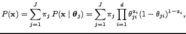
The mixture model used in the BernoulliMix package is a finite mixture model of multivariate Bernoulli distributions [Wolfe, 1970], solely concentrating on modeling of 0-1 (zero-one) data. The likelihood of the observed data is readily calculated with

$$P(\mathbf{x}) = \sum_{j=1}^J \pi_j\, P(\mathbf{x} \mid \boldsymbo... ..._{j=1}^J \pi_j \prod_{i=1}^{d} \theta_{ji}^{x_i}(1 - \theta_{ji})^{1 - x_i},$$

where the data vector is $\mathbf{x} = (x_1, \ldots, x_d)$, the data is binary $x_i \in \{0,1\}$ and the mixture model is parameterized by the mixing coefficients $\pi_j, j=1,\ldots, J$ and the parameters for the component distributions $\boldsymbol{\theta}_j = (\theta_{j1}, \theta_{j2}, \ldots, \theta_{jd})$, $\theta_{ij} \in [0,1]$